import numpy as np
import matplotlib.pyplot as plt
from utils import *

%matplotlib inlineAnomaly Computer Servers
Let’s implement an anomaly detection algorithm to detect anomalous behavior in server computers.
The dataset contains two features -
- throughput (mb/s) and
- latency (ms) of response of each server.
While your servers were operating, you collected 𝑚=307m=307 examples of how they were behaving, and thus have an unlabeled dataset {𝑥(1),…,𝑥(𝑚)}{x(1),…,x(m)}.
- You suspect that the vast majority of these examples are “normal” (non-anomalous) examples of the servers operating normally, but there might also be some examples of servers acting anomalously within this dataset.
You will use a Gaussian model to detect anomalous examples in your dataset.
- You will first start on a 2D dataset that will allow you to visualize what the algorithm is doing.
- On that dataset you will fit a Gaussian distribution and then find values that have very low probability and hence can be considered anomalies.
- After that, you will apply the anomaly detection algorithm to a larger dataset with many dimensions.
Data
The load_data() function shown below loads the data into the variables X_train, X_val and y_val
- You will use
X_trainto fit a Gaussian distribution - You will use
X_valandy_valas a cross validation set to select a threshold and determine anomalous vs normal examples
# Load the dataset
X_train, X_val, y_val = load_data()
# Display the first five elements of X_train
print("The first 5 elements of X_train are:\n", X_train[:5])
# Display the first five elements of X_val
print("The first 5 elements of X_val are\n", X_val[:5])
# Display the first five elements of y_val
print("The first 5 elements of y_val are\n", y_val[:5]) 
print ('The shape of X_train is:', X_train.shape)
print ('The shape of X_val is:', X_val.shape)
print ('The shape of y_val is: ', y_val.shape)
The shape of X_train is: (307, 2)
The shape of X_val is: (307, 2)
The shape of y_val is: (307,)Before starting on any task, it is often useful to understand the data by visualizing it.
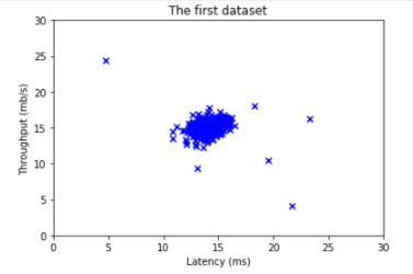
- For this dataset, you can use a scatter plot to visualize the data (
X_train), since it has only two properties to plot (throughput and latency) - Your plot should look similar to the one below
# Create a scatter plot of the data. To change the markers to blue "x",
# we used the 'marker' and 'c' parameters
plt.scatter(X_train[:, 0], X_train[:, 1], marker='x', c='b')

# Set the title
plt.title("The first dataset")
# Set the y-axis label
plt.ylabel('Throughput (mb/s)')
# Set the x-axis label
plt.xlabel('Latency (ms)')
# Set axis range
plt.axis([0, 30, 0, 30])
plt.show()
Gaussian DIstribution
Fit model to the data’s distributio
- Given a training set {𝑥(1),…,𝑥(𝑚)}{x(1),…,x(m)} you want to estimate the Gaussian distribution for each of the features 𝑥𝑖xi.
- Recall that the Gaussian distribution is given by

- where 𝜇μ is the mean and 𝜎2σ2 is the variance.
- For each feature 𝑖=1…𝑛i=1…n, you need to find parameters 𝜇𝑖μi and 𝜎2𝑖σi2 that fit the data in the 𝑖i-th dimension {𝑥(1)𝑖,…,𝑥(𝑚)𝑖}{xi(1),…,xi(m)} (the 𝑖i-th dimension of each example).
Estimate the parameters ( \(\mu\) i, \(\sigma\) i2) of the i-th feature by using the following equations.
Estimate the mean

and for the variance you will use

def estimate_gaussian(X):
    """
    Calculates mean and variance of all features
    in the dataset

    Args:
        X (ndarray): (m, n) Data matrix

    Returns:
        mu (ndarray): (n,) Mean of all features
        var (ndarray): (n,) Variance of all features
    """

    m, n = X.shape

    mu = 1 / m * np.sum(X, axis = 0)
    var = 1 / m * np.sum((X - mu) ** 2, axis = 0)

    return mu, var
# Estimate mean and variance of each feature
mu, var = estimate_gaussian(X_train)
print("Mean of each feature:", mu)
print("Variance of each feature:", var)Mean of each feature: [14.11222578 14.99771051]
Variance of each feature: [1.83263141 1.70974533]Visualize Gaussian Distribution
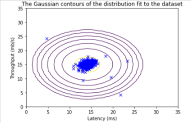
# Returns the density of the multivariate normal
# at each data point (row) of X_train
p = multivariate_gaussian(X_train, mu, var)

#Plotting code
visualize_fit(X_train, mu, var)
Select Threshold
Now that you have estimated the Gaussian parameters, you can investigate which examples have a very high probability given this distribution and which examples have a very low probability.
- The low probability examples are more likely to be the anomalies in our dataset.
- One way to determine which examples are anomalies is to select a threshold based on a cross validation set.
In this section, you will complete the code in select_threshold to select the threshold 𝜀ε using the 𝐹1F1 score on a cross validation set.
- For this, we will use a cross validation set {(𝑥(1)cv,𝑦(1)cv),…,(𝑥(𝑚cv)cv,𝑦(𝑚cv)cv)}{(xcv(1),ycv(1)),…,(xcv(mcv),ycv(mcv))}, where the label 𝑦=1y=1 corresponds to an anomalous example, and 𝑦=0y=0 corresponds to a normal example.
- For each cross validation example, we will compute 𝑝(𝑥(𝑖)cv)p(xcv(i)). The vector of all of these probabilities 𝑝(𝑥(1)cv),…,𝑝(𝑥(𝑚cv)cv)p(xcv(1)),…,p(xcv(mcv)) is passed to
select_thresholdin the vectorp_val. - The corresponding labels 𝑦(1)cv,…,𝑦(𝑚cv)cvycv(1),…,ycv(mcv) are passed to the same function in the vector
y_val.
Function Below
To find the best threshold to use for selecting outliers based on the results from the validation set (p_val) and the ground truth (y_val).
- In the provided code
select_threshold, there is already a loop that will try many different values of 𝜀ε and select the best 𝜀ε based on the 𝐹1F1 score. - You need to implement code to calculate the F1 score from choosing
epsilonas the threshold and place the value inF1.Recall that if an example 𝑥x has a low probability 𝑝(𝑥)<𝜀p(x)<ε, then it is classified as an anomaly.
Then, you can compute precision and recall by:

where
- 𝑡𝑝tp is the number of true positives: the ground truth label says it’s an anomaly and our algorithm correctly classified it as an anomaly.
- 𝑓𝑝fp is the number of false positives: the ground truth label says it’s not an anomaly, but our algorithm incorrectly classified it as an anomaly.
- 𝑓𝑛fn is the number of false negatives: the ground truth label says it’s an anomaly, but our algorithm incorrectly classified it as not being anomalous.
- The 𝐹1F1 score is computed using precision (𝑝𝑟𝑒𝑐prec) and recall (𝑟𝑒𝑐rec) as follows:

NOTE
- If you have several binary values in an 𝑛n-dimensional binary vector, you can find out how many values in this vector are 0 by using: `np.sum(v == 0)`
- You can also apply a logical *and* operator to such binary vectors. For instance, `predictions` is a binary vector of the size of your number of cross validation set, where the 𝑖i-th element is 1 if your algorithm considers 𝑥(𝑖)cvxcv(i) an anomaly, and 0 otherwise.
- You can then, for example, compute the number of false positives using:
fp = sum((predictions == 1) & (y_val == 0))
def select_threshold(y_val, p_val):
    """
    Finds the best threshold to use for selecting outliers
    based on the results from a validation set (p_val)
    and the ground truth (y_val)

    Args:
        y_val (ndarray): Ground truth on validation set
        p_val (ndarray): Results on validation set

    Returns:
        epsilon (float): Threshold chosen
        F1 (float):      F1 score by choosing epsilon as threshold
    """

    best_epsilon = 0
    best_F1 = 0
    F1 = 0

    step_size = (max(p_val) - min(p_val)) / 1000

    for epsilon in np.arange(min(p_val), max(p_val), step_size):
       predictions = (p_val < epsilon)

       # calculate number of true positives
       tp = np.sum((predictions == 1) & (y_val == 1))
       # calculate number of false positives
       fp = sum((predictions == 1) & (y_val == 0))
       # Your code here to calculate number of false negatives
       fn = np.sum((predictions == 0) & (y_val == 1))


       # calculate precision
       prec = tp / (tp + fp)
       # calculate recall
       rec = tp / (tp+fn)
       # calculate F1
       F1 = 2 * prec * rec / (prec + rec)

       if F1 > best_F1:
           best_F1 = F1
           best_epsilon = epsilon

    return best_epsilon, best_F1
p_val = multivariate_gaussian(X_val, mu, var)
epsilon, F1 = select_threshold(y_val, p_val)
print('Best epsilon found using cross-validation: %e' % epsilon)
print('Best F1 on Cross Validation Set: %f' % F1)Best epsilon found using cross-validation: 8.990853e-05
Best F1 on Cross Validation Set: 0.875000Detect Anomaly
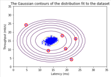
Run anomaly detection code and circle the anomalies in the plot

Real Data Test
Now, we will run the anomaly detection algorithm that you implemented on a more realistic and much harder dataset.
In this dataset, each example is described by 11 features, capturing many more properties of your compute servers.
Let’s start by loading the dataset.
- The
load_data()function shown below loads the data into variablesX_train_high,X_val_highandy_val_high _highis meant to distinguish these variables from the ones used in the previous part- We will use
X_train_highto fit Gaussian distribution - We will use
X_val_highandy_val_highas a cross validation set to select a threshold and determine anomalous vs normal examples
# load the dataset
X_train_high, X_val_high, y_val_high = load_data_multi()
print ('The shape of X_train_high is:', X_train_high.shape)
print ('The shape of X_val_high is:', X_val_high.shape)
print ('The shape of y_val_high is: ', y_val_high.shape)The shape of X_train_high is: (1000, 11)
The shape of X_val_high is: (100, 11)
The shape of y_val_high is: (100,)Detect Anomaly
Let’s run the anomaly algorithm on the new dataset. Here are the steps
- Estimate the Gaussian parameters (𝜇𝑖μi and 𝜎2𝑖σi2)
- Evaluate the probabilities for both the training data
X_train_highfrom which you estimated the Gaussian parameters, as well as for the the cross-validation setX_val_high. - Finally, it will use
select_thresholdto find the best threshold 𝜀ε.
# Apply the same steps to the larger dataset

# Estimate the Gaussian parameters
mu_high, var_high = estimate_gaussian(X_train_high)

# Evaluate the probabilites for the training set
p_high = multivariate_gaussian(X_train_high, mu_high, var_high)

# Evaluate the probabilites for the cross validation set
p_val_high = multivariate_gaussian(X_val_high, mu_high, var_high)

# Find the best threshold
epsilon_high, F1_high = select_threshold(y_val_high, p_val_high)

print('Best epsilon found using cross-validation: %e'% epsilon_high)
print('Best F1 on Cross Validation Set:  %f'% F1_high)
print('# Anomalies found: %d'% sum(p_high < epsilon_high))
Best epsilon found using cross-validation: 1.377229e-18
Best F1 on Cross Validation Set: 0.615385
# Anomalies found: 117