import numpy as np
import matplotlib.pyplot as plt
from utils import *

%matplotlib inlineImage Compression K-means
- In a straightforward 24-bit color representation of an image22, each pixel is represented as three 8-bit unsigned integers (ranging from 0 to 255) that specify the red, green and blue intensity values. This encoding is often refered to as the RGB encoding.
- Our image contains thousands of colors, and in this part of the exercise, you will reduce the number of colors to 16 colors.
- By making this reduction, it is possible to represent (compress) the photo in an efficient way.
- Specifically, you only need to store the RGB values of the 16 selected colors, and for each pixel in the image you now need to only store the index of the color at that location (where only 4 bits are necessary to represent 16 possibilities).
We will use the K-means algorithm to select the 16 colors that will be used to represent the compressed image.
- Concretely, we will treat every pixel in the original image as a data example and use the K-means algorithm to find the 16 colors that best group (cluster) the pixels in the 3- dimensional RGB space.
- Once we have computed the cluster centroids on the image, we will then use the 16 colors to replace the pixels in the original image.
Here is the original 128X128 image
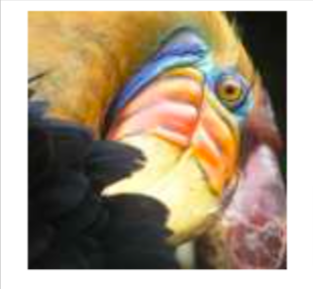
.
Load Image
# Load an image of a bird
original_img = plt.imread('bird_small.png')
# Visualizing the image
plt.imshow(original_img)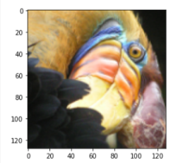
print("Shape of original_img is:", original_img.shape)
This is a 3-D matrix where
- the first 2 indices identify a pixel position and
- the third index represents red, green, or blue
- for example orginal_img(20,33,2) gives the blue intensity of the pixel at row 50 and column33
Transform to 2D
Let’s first transform the matrix to 2D matrix
- The code below reshapes the matrix
original_imgto create an 𝑚×3m×3 matrix of pixel colors (where 𝑚=16384=128×128m=16384=128×128)
Note: If you’ll try this exercise later on a JPG file, you first need to divide the pixel values by 255 so it will be in the range 0 to 1. This is not necessary for PNG files (e.g. bird_small.png) because it is already loaded in the required range (as mentioned in the plt.imread() documentation). We commented a line below for this so you can just uncomment it later in case you want to try a different file.
# Divide by 255 so that all values are in the range 0 - 1 (not needed for PNG files)
# original_img = original_img / 255

# Reshape the image into an m x 3 matrix where m = number of pixels
# (in this case m = 128 x 128 = 16384)
# Each row will contain the Red, Green and Blue pixel values
# This gives us our dataset matrix X_img that we will use K-Means on.

X_img = np.reshape(original_img, (original_img.shape[0] * original_img.shape[1], 3))
Run K-means
Let’s run k-means on the pre-processed image
# Run your K-Means algorithm on this data
# You should try different values of K and max_iters here
K = 16
max_iters = 10

# Using the function you have implemented above.
initial_centroids = kMeans_init_centroids(X_img, K)

# Run K-Means - this can take a couple of minutes depending on K and max_iters
centroids, idx = run_kMeans(X_img, initial_centroids, max_iters)
print("Shape of idx:", idx.shape)
print("Closest centroid for the first five elements:", idx[:5])
Shape of idx: (16384,)
Closest centroid for the first five elements: [4 4 4 4 4]Plot colors
The code below will plot all the colors found in the original image. As mentioned earlier, the color of each pixel is represented by RGB values so the plot should have 3 axes – R, G, and B. You’ll notice a lot of dots below representing thousands of colors in the original image. The red markers represent the centroids after running K-means. These will be the 16 colors that you will use to compress the image.
# Plot the colors of the image and mark the centroids
plot_kMeans_RGB(X_img, centroids, idx, K)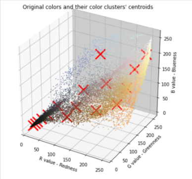
You can visualize the colors at each of the red markers (i.e. the centroids) above with the function below. You will only see these colors when you generate the new image in the next section. The number below each color is its index and these are the numbers you see in the idx array.
# Visualize the 16 colors selected
show_centroid_colors(centroids)
Compress Image
After finding the top 𝐾=16K=16 colors to represent the image, you can now assign each pixel position to its closest centroid using the find_closest_centroids function.
- This allows you to represent the original image using the centroid assignments of each pixel.
- Notice that you have significantly reduced the number of bits that are required to describe the image.
The original image required 24 bits (i.e. 8 bits x 3 channels in RGB encoding) for each one of the 128×128128×128 pixel locations, resulting in total size of 128×128×24=393,216128×128×24=393,216 bits.
The new representation requires some overhead storage in form of a dictionary of 16 colors, each of which require 24 bits, but the image itself then only requires 4 bits per pixel location.
The final number of bits used is therefore 16×24+128×128×4=65,92016×24+128×128×4=65,920 bits, which corresponds to compressing the original image by about a factor of 6.
# Find the closest centroid of each pixel
idx = find_closest_centroids(X_img, centroids)

# Replace each pixel with the color of the closest centroid
X_recovered = centroids[idx, :]

# Reshape image into proper dimensions
X_recovered = np.reshape(X_recovered, original_img.shape)
View Image
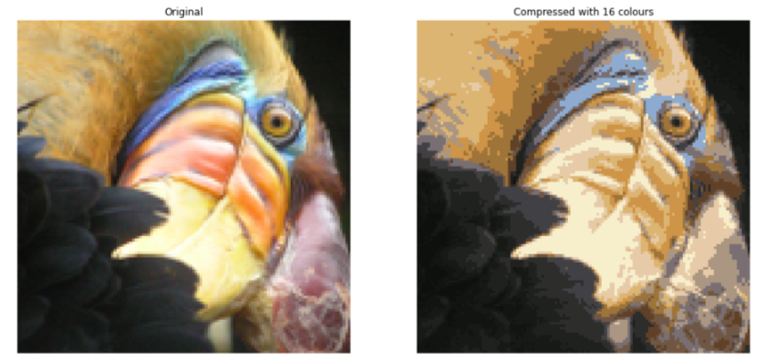
Finally, you can view the effects of the compression by reconstructing the image based only on the centroid assignments.
- Specifically, you replaced each pixel with the value of the centroid assigned to it.
- Figure shows a sample reconstruction. Even though the resulting image retains most of the characteristics of the original, you will also see some compression artifacts because of the fewer colors used.
# Display original image
fig, ax = plt.subplots(1,2, figsize=(16,16))
plt.axis('off')

ax[0].imshow(original_img)
ax[0].set_title('Original')
ax[0].set_axis_off()


# Display compressed image
ax[1].imshow(X_recovered)
ax[1].set_title('Compressed with %d colours'%K)
ax[1].set_axis_off()