import numpy as np
import tensorflow as tf
from tensorflow.keras.models import Sequential
from tensorflow.keras.layers import Dense
import matplotlib.pyplot as plt
from autils import *
%matplotlib inline

import logging
logging.getLogger("tensorflow").setLevel(logging.ERROR)
tf.autograph.set_verbosity(0)NN Digit Recognition I
We will use a NN to recognize the hand-written digits: zero and one. This is a binary classification task. Automated handwritten digit recognition is widely used today - from recognizing zip codes (postal codes) on mail envelopes to recognizing amounts written on bank checks.
Setup
- Tensorflow is a machine learning package developed by Google. In 2019, Google integrated Keras into Tensorflow and released Tensorflow 2.0.
- Keras is a framework developed independently by François Chollet that creates a simple, layer-centric interface to Tensorflow.
.
Dataset
Wewill start by loading the dataset for this task.
- The
load_data()function shown below loads the data into variablesXandy - The data set contains 1000 training examples of handwritten digits 1, here limited to zero and one.
Each training example is a 20-pixel x 20-pixel grayscale image of the digit.
Each pixel is represented by a floating-point number indicating the grayscale intensity at that location.
The 20 by 20 grid of pixels is “unrolled” into a 400-dimensional vector.
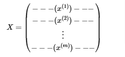
Each training example becomes a single row in our data matrix
X.This gives us a 1000 x 400 matrix
Xwhere every row is a training example of a handwritten digit image.
- The second part of the training set is a 1000 x 1 dimensional vector
ythat contains labels for the training sety = 0if the image is of the digit0,y = 1if the image is of the digit1.
- This is a subset of the MNIST handwritten digit dataset (http://yann.lecun.com/exdb/mnist/)
# load dataset
X, y = load_data()
View Data
print ('The first element of X is: ', X[0])
print ('The first element of y is: ', y[0,0])
print ('The last element of y is: ', y[-1,0])
print ('The shape of X is: ' + str(X.shape))
print ('The shape of y is: ' + str(y.shape))
Plot
We will begin by visualizing a subset of the training set.
- In the cell below, the code randomly selects 64 rows from
X, maps each row back to a 20 pixel by 20 pixel grayscale image and displays the images together. - The label for each image is displayed above the image
import warnings
warnings.simplefilter(action='ignore', category=FutureWarning)
# You do not need to modify anything in this cell

m, n = X.shape

fig, axes = plt.subplots(8,8, figsize=(8,8))
fig.tight_layout(pad=0.1)

for i,ax in enumerate(axes.flat):
    # Select random indices
    random_index = np.random.randint(m)

    # Select rows corresponding to the random indices and
    # reshape the image
    X_random_reshaped = X[random_index].reshape((20,20)).T

    # Display the image
    ax.imshow(X_random_reshaped, cmap='gray')

    # Display the label above the image
    ax.set_title(y[random_index,0])
    ax.set_axis_off()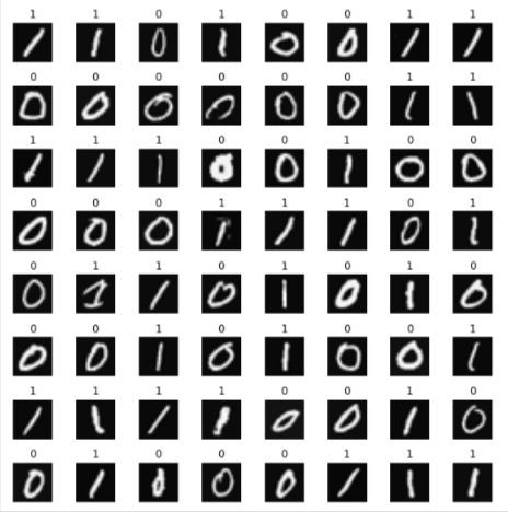
Create Model
The neural network you will use in this assignment is shown in the figure below.
- This has three dense layers with sigmoid activations.
Recall that our inputs are pixel values of digit images.
Since the images are of size 20×20, this gives us 400 inputs
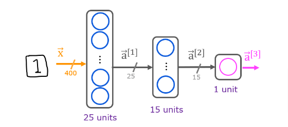
- The parameters have dimensions that are sized for a neural network with 2525 units in layer 1, 1515 units in layer 2 and 11 output unit in layer 3.
Recall that the dimensions of these parameters are determined as follows:
If network has 𝑠𝑖𝑛sin units in a layer and 𝑠𝑜𝑢𝑡sout units in the next layer, then
𝑊W will be of dimension 𝑠𝑖𝑛×𝑠𝑜𝑢𝑡sin×sout.
𝑏b will a vector with 𝑠𝑜𝑢𝑡sout elements
Therefore, the shapes of
W, andb, arelayer1: The shape of
W1is (400, 25) and the shape ofb1is (25,)layer2: The shape of
W2is (25, 15) and the shape ofb2is: (15,)layer3: The shape of
W3is (15, 1) and the shape ofb3is: (1,)Note: The bias vector
bcould be represented as a 1-D (n,) or 2-D (1,n) array. Tensorflow utilizes a 1-D representation and this lab will maintain that convention.
Tensorflow
Tensorflow models are built layer by layer. A layer’s input dimensions (𝑠𝑖𝑛sin above) are calculated for you. You specify a layer’s output dimensions and this determines the next layer’s input dimension. The input dimension of the first layer is derived from the size of the input data specified in the model.fit statement below.
Note: It is also possible to add an input layer that specifies the input dimension of the first layer. For example:
tf.keras.Input(shape=(400,)), #specify input shape
We will include that here to illuminate some model sizing.
Construct Network
We’ll be using Keras Sequential model and Dense Layer with a sigmoid activation to construct the network described above
model = Sequential(
    [
        tf.keras.Input(shape=(400,)),    #specify input size
        Dense(25, activation='sigmoid', name = 'layer1'),
        Dense(15, activation='sigmoid', name = 'layer2'),
        Dense(1, activation='sigmoid', name = 'layer3')
    ], name = "my_model"
)
or we can omit the layers like this
model = Sequential(
    [
        tf.keras.Input(shape=(400,)),    #specify input size
        Dense(25, activation='sigmoid'),
        Dense(15, activation='sigmoid'),
        Dense(1, activation='sigmoid')
    ], name = "my_model"
)
Review
model.summary()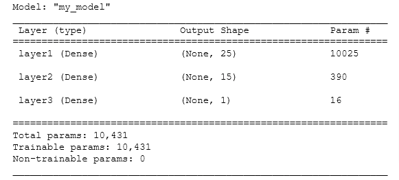
Parameters & Counts
L1_num_params = 400 * 25 + 25  # W1 parameters  + b1 parameters
L2_num_params = 25 * 15 + 15   # W2 parameters  + b2 parameters
L3_num_params = 15 * 1 + 1     # W3 parameters  + b3 parameters
print("L1 params = ", L1_num_params, ", L2 params = ", L2_num_params, ",  L3 params = ", L3_num_params )
Extract Layers
[layer1, layer2, layer3] = model.layersExtract Shape
#### Examine Weights shapes
W1,b1 = layer1.get_weights()
W2,b2 = layer2.get_weights()
W3,b3 = layer3.get_weights()
print(f"W1 shape = {W1.shape}, b1 shape = {b1.shape}")
print(f"W2 shape = {W2.shape}, b2 shape = {b2.shape}")
print(f"W3 shape = {W3.shape}, b3 shape = {b3.shape}")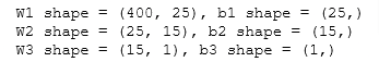
Extract Weights
xx.get_weights returns a NumPy array. One can also access the weights directly in their tensor form. Note the shape of the tensors in the final layer.
print(model.layers[2].weights)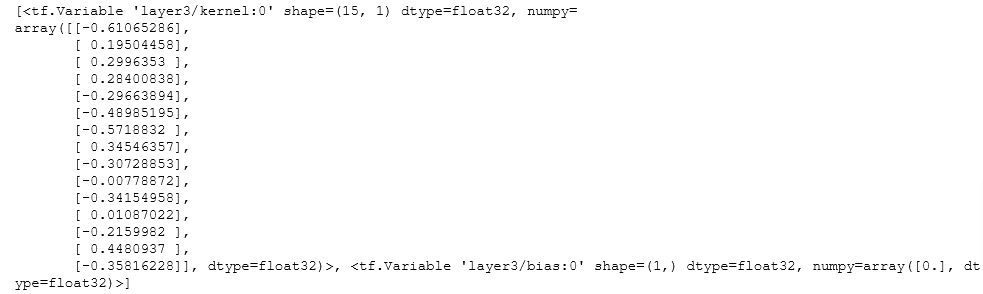
Loss Function
Compile the model
Gradient Descent
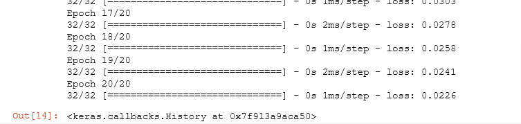
Train the model by running the loss function and GD to fit the weights of the model to the training data.
model.compile(
    loss=tf.keras.losses.BinaryCrossentropy(),
    optimizer=tf.keras.optimizers.Adam(0.001),
)

model.fit(
    X,y,
    epochs=20
)
Predict
- To run the model on an example to make a prediction, use Keras
predict. - The input to
predictis an array so the single example is reshaped to be two dimensional. - In the first example below, the number is 0, so the model predicts the probability that the input is a ONE is nearly zero: 0.01301..
- Then in the second example the number is a one and the model predicts that the probability that it is a ONE as nearly one
- Then we compare the probability to a threshold to make a final prediction
prediction = model.predict(X[0].reshape(1,400))  # a zero as input
print(f" predicting a zero: {prediction}")
prediction = model.predict(X[500].reshape(1,400))  # a one as input
print(f" predicting a one:  {prediction}")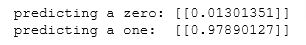
if prediction >= 0.5:
    yhat = 1
else:
    yhat = 0
print(f"prediction after threshold: {yhat}")
Predict Random Input
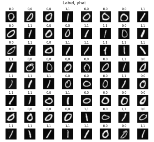
Let’s compare the predictions vs the labels for a random sample of 64 digits. This takes a moment to run.
import warnings
warnings.simplefilter(action='ignore', category=FutureWarning)
# You do not need to modify anything in this cell

m, n = X.shape

fig, axes = plt.subplots(8,8, figsize=(8,8))
fig.tight_layout(pad=0.1,rect=[0, 0.03, 1, 0.92]) #[left, bottom, right, top]

for i,ax in enumerate(axes.flat):
    # Select random indices
    random_index = np.random.randint(m)

    # Select rows corresponding to the random indices and
    # reshape the image
    X_random_reshaped = X[random_index].reshape((20,20)).T

    # Display the image
    ax.imshow(X_random_reshaped, cmap='gray')

    # Predict using the Neural Network
    prediction = model.predict(X[random_index].reshape(1,400))
    if prediction >= 0.5:
        yhat = 1
    else:
        yhat = 0

    # Display the label above the image
    ax.set_title(f"{y[random_index,0]},{yhat}")
    ax.set_axis_off()
fig.suptitle("Label, yhat", fontsize=16)
plt.show()