Data

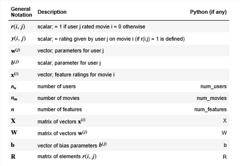
Notations

The diagram below details how these vectors are learned.

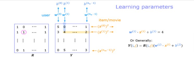
Existing ratings are provided in matrix form as shown.

𝑌Y contains ratings; 0.5 to 5 inclusive in 0.5 steps. 0 if the movie has not been rated. 𝑅R has a 1 where movies have been rated.
Movies are in rows, users in columns. Each user has a parameter vector 𝑤𝑢𝑠𝑒𝑟wuser and bias.
Each movie has a feature vector 𝑥𝑚𝑜𝑣𝑖𝑒xmovie. These vectors are simultaneously learned by using the existing user/movie ratings as training data.
One training example is shown above: 𝐰(1)⋅𝐱(1)+𝑏(1)=4w(1)⋅x(1)+b(1)=4.
It is worth noting that the feature vector 𝑥𝑚𝑜𝑣𝑖𝑒xmovie must satisfy all the users while the user vector 𝑤𝑢𝑠𝑒𝑟wuser must satisfy all the movies.
This is the source of the name of this approach - all the users collaborate to generate the rating set.

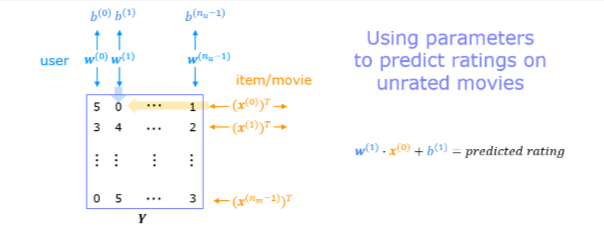
Once the feature vectors and parameters are learned, they can be used to predict how a user might rate an unrated movie.
This is shown in the diagram above. The equation is an example of predicting a rating for user 1 on movie 0

Dataset

The data set is derived from the MovieLens “ml-latest-small” dataset.
[F. Maxwell Harper and Joseph A. Konstan. 2015. The MovieLens Datasets: History and Context. ACM Transactions on Interactive Intelligent Systems (TiiS) 5, 4: 19:1–19:19. https://doi.org/10.1145/2827872]

The original dataset has 9000 movies rated by 600 users. The dataset has been reduced in size to focus on movies from the years since 2000. This dataset consists of ratings on a scale of 0.5 to 5 in 0.5 step increments. The reduced dataset has 𝑛𝑢=443nu=443 users, and 𝑛𝑚=4778nm=4778 movies.

Below, you will load the movie dataset into the variables 𝑌Y and 𝑅R.

The matrix 𝑌Y (a 𝑛𝑚×𝑛𝑢nm×nu matrix) stores the ratings 𝑦(𝑖,𝑗)y(i,j).
The matrix 𝑅R is an binary-valued indicator matrix, where 𝑅(𝑖,𝑗)=1R(i,j)=1 if user 𝑗j gave a rating to movie 𝑖i, and 𝑅(𝑖,𝑗)=0R(i,j)=0 otherwise.

Throughout this part of the exercise, you will also be working with the matrices, 𝐗X, 𝐖W and 𝐛b:

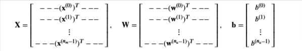
The 𝑖i-th row of 𝐗X corresponds to the feature vector 𝑥(𝑖)x(i) for the 𝑖i-th movie, and the 𝑗j-th row of 𝐖W corresponds to one parameter vector 𝐰(𝑗)w(j), for the 𝑗j-th user.
Both 𝑥(𝑖)x(i) and 𝐰(𝑗)w(j) are 𝑛n-dimensional vectors. For the purposes of this exercise, you will use 𝑛=10n=10, and therefore, 𝐱(𝑖)x(i) and 𝐰(𝑗)w(j) have 10 elements. Correspondingly, 𝐗X is a 𝑛𝑚×10nm×10 matrix and 𝐖W is a 𝑛𝑢×10nu×10 matrix.

Setup

import numpy as np
import tensorflow as tf
from tensorflow import keras
from recsys_utils import *

Load Data

We will start by loading the movie ratings dataset to understand the structure of the data. We will load 𝑌Y and 𝑅R with the movie dataset.
We’ll also load 𝐗X, 𝐖W, and 𝐛b with pre-computed values. These values will be learned later in the lab, but we’ll use pre-computed values to develop the cost model.

#Load data
X, W, b, num_movies, num_features, num_users = load_precalc_params_small()
Y, R = load_ratings_small()

print("Y", Y.shape, "R", R.shape)
print("X", X.shape)
print("W", W.shape)
print("b", b.shape)
print("num_features", num_features)
print("num_movies",   num_movies)
print("num_users",    num_users)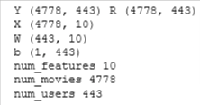

Calculate Mean

#  From the matrix, we can compute statistics like average rating.
tsmean =  np.mean(Y[0, R[0, :].astype(bool)])
print(f"Average rating for movie 1 : {tsmean:0.3f} / 5" )

Collaborative Filtering

We will begin implementing the collaborative filtering learning algorithm. You will start by implementing the objective function.

The collaborative filtering algorithm in the setting of movie recommendations considers a set of 𝑛n-dimensional parameter vectors 𝐱(0),…,𝐱(𝑛𝑚−1)x(0),…,x(nm−1), 𝐰(0),…,𝐰(𝑛𝑢−1)w(0),…,w(nu−1) and 𝑏(0),…,𝑏(𝑛𝑢−1)b(0),…,b(nu−1)
where the model predicts the rating for movie 𝑖i by user 𝑗j as 𝑦(𝑖,𝑗)=𝐰(𝑗)⋅𝐱(𝑖)+𝑏(𝑗)y(i,j)=w(j)⋅x(i)+b(j)
Given a dataset that consists of a set of ratings produced by some users on some movies, you wish to learn the parameter vectors 𝐱(0),…,𝐱(𝑛𝑚−1),𝐰(0),…,𝐰(𝑛𝑢−1)x(0),…,x(nm−1),w(0),…,w(nu−1)
and 𝑏(0),…,𝑏(𝑛𝑢−1)b(0),…,b(nu−1)
that produce the best fit (minimizes the squared error).

Cost Function

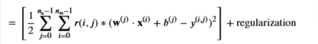
Compute the cost function for collaborative filtering.

The first summation in (1) is for all i, j where r(i,j) equals 1 and could be written as

def cofi_cost_func(X, W, b, Y, R, lambda_):
    """
    Returns the cost for the content-based filtering
    Args:
      X (ndarray (num_movies,num_features)): matrix of item features
      W (ndarray (num_users,num_features)) : matrix of user parameters
      b (ndarray (1, num_users)            : vector of user parameters
      Y (ndarray (num_movies,num_users)    : matrix of user ratings of movies
      R (ndarray (num_movies,num_users)    : matrix, where R(i, j) = 1 if the i-th movies was rated by the j-th user
      lambda_ (float): regularization parameter
    Returns:
      J (float) : Cost
    """
    nm,nu = Y.shape
    J = 0
      
    for j in range(nu):
        w = W[j,:]
        b_j = b[0,j]
        for i in range(nm):
            x = X[i,:]
            y = Y[i,j]
            r = R[i,j]
            J += np.square(r * (np.dot(w,x) + b_j - y ) )
    J = J/2
    J += (lambda_/2) * (np.sum(np.square(W)) + np.sum(np.square(X)))

    return J

Reduce Dataset

# Reduce the data set size so that this runs faster
num_users_r = 4
num_movies_r = 5 
num_features_r = 3

X_r = X[:num_movies_r, :num_features_r]
W_r = W[:num_users_r,  :num_features_r]
b_r = b[0, :num_users_r].reshape(1,-1)
Y_r = Y[:num_movies_r, :num_users_r]
R_r = R[:num_movies_r, :num_users_r]

# Evaluate cost function
J = cofi_cost_func(X_r, W_r, b_r, Y_r, R_r, 0);
print(f"Cost: {J:0.2f}")

Cost: 13.67

Regularization

# Evaluate cost function with regularization 
J = cofi_cost_func(X_r, W_r, b_r, Y_r, R_r, 1.5);
print(f"Cost (with regularization): {J:0.2f}")

Cost (with regularization): 28.09

Vectorized Implementation

It is important to create a vectorized implementation to compute 𝐽J, since it will later be called many times during optimization. The linear algebra utilized is not the focus of this series, so the implementation is provided. If you are an expert in linear algebra, feel free to create your version without referencing the code below.

def cofi_cost_func_v(X, W, b, Y, R, lambda_):
    """
    Returns the cost for the content-based filtering
    Vectorized for speed. Uses tensorflow operations to be compatible with custom training loop.
    Args:
      X (ndarray (num_movies,num_features)): matrix of item features
      W (ndarray (num_users,num_features)) : matrix of user parameters
      b (ndarray (1, num_users)            : vector of user parameters
      Y (ndarray (num_movies,num_users)    : matrix of user ratings of movies
      R (ndarray (num_movies,num_users)    : matrix, where R(i, j) = 1 if the i-th movies was rated by the j-th user
      lambda_ (float): regularization parameter
    Returns:
      J (float) : Cost
    """
    j = (tf.linalg.matmul(X, tf.transpose(W)) + b - Y)*R
    J = 0.5 * tf.reduce_sum(j**2) + (lambda_/2) * (tf.reduce_sum(X**2) + tf.reduce_sum(W**2))
    return J

Evaluate Cost Function

# Evaluate cost function
J = cofi_cost_func_v(X_r, W_r, b_r, Y_r, R_r, 0);
print(f"Cost: {J:0.2f}")

# Evaluate cost function with regularization 
J = cofi_cost_func_v(X_r, W_r, b_r, Y_r, R_r, 1.5);
print(f"Cost (with regularization): {J:0.2f}")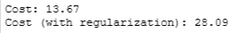

Train Algorithm

Now that we have the collaborative filtering cost function, we can start training our algorithm to make movie recommendations based on our choices.

So let’s enter our own movie choices, the algorithm will then make recommendations. So I went ahead and made some choices.

movieList, movieList_df = load_Movie_List_pd()

my_ratings = np.zeros(num_movies)          #  Initialize my ratings

# Check the file small_movie_list.csv for id of each movie in our dataset
# For example, Toy Story 3 (2010) has ID 2700, so to rate it "5", you can set
my_ratings[2700] = 5 

#Or suppose you did not enjoy Persuasion (2007), you can set
my_ratings[2609] = 2;

# We have selected a few movies we liked / did not like and the ratings we
# gave are as follows:
my_ratings[929]  = 5   # Lord of the Rings: The Return of the King, The
my_ratings[246]  = 5   # Shrek (2001)
my_ratings[2716] = 3   # Inception
my_ratings[1150] = 5   # Incredibles, The (2004)
my_ratings[382]  = 2   # Amelie (Fabuleux destin d'Amélie Poulain, Le)
my_ratings[366]  = 5   # Harry Potter and the Sorcerer's Stone (a.k.a. Harry Potter and the Philosopher's Stone) (2001)
my_ratings[622]  = 5   # Harry Potter and the Chamber of Secrets (2002)
my_ratings[988]  = 3   # Eternal Sunshine of the Spotless Mind (2004)
my_ratings[2925] = 1   # Louis Theroux: Law & Disorder (2008)
my_ratings[2937] = 1   # Nothing to Declare (Rien à déclarer)
my_ratings[793]  = 5   # Pirates of the Caribbean: The Curse of the Black Pearl (2003)
my_rated = [i for i in range(len(my_ratings)) if my_ratings[i] > 0]

print('\nNew user ratings:\n')
for i in range(len(my_ratings)):
    if my_ratings[i] > 0 :
        print(f'Rated {my_ratings[i]} for  {movieList_df.loc[i,"title"]}');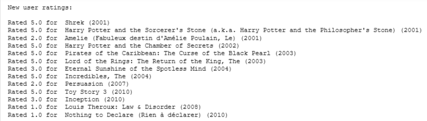

Add Our Reviews to Y and R and normalize the ratings

# Reload ratings
Y, R = load_ratings_small()

# Add new user ratings to Y 
Y = np.c_[my_ratings, Y]

# Add new user indicator matrix to R
R = np.c_[(my_ratings != 0).astype(int), R]

# Normalize the Dataset
Ynorm, Ymean = normalizeRatings(Y, R)

Retrain with Added Data

#  Useful Values
num_movies, num_users = Y.shape
num_features = 100

# Set Initial Parameters (W, X), use tf.Variable to track these variables
tf.random.set_seed(1234) # for consistent results
W = tf.Variable(tf.random.normal((num_users,  num_features),dtype=tf.float64),  name='W')
X = tf.Variable(tf.random.normal((num_movies, num_features),dtype=tf.float64),  name='X')
b = tf.Variable(tf.random.normal((1,          num_users),   dtype=tf.float64),  name='b')

# Instantiate an optimizer.
optimizer = keras.optimizers.Adam(learning_rate=1e-1)

Let’s now train the collaborative filtering model. This will learn the parameters 𝐗X, 𝐖W, and 𝐛b.

The operations involved in learning 𝑤w, 𝑏b, and 𝑥x simultaneously do not fall into the typical ‘layers’ offered in the TensorFlow neural network package. Consequently, the flow used in Course 2: Model, Compile(), Fit(), Predict(), are not directly applicable. Instead, we can use a custom training loop.

Recall from before

repeat until convergence:
- compute forward pass
- compute the derivatives of the loss relative to parameters
- update the parameters using the learning rate and the computed derivatives

TensorFlow has the capability of calculating the derivatives for you. This is shown below.

Within the tf.GradientTape() section, operations on Tensorflow Variables are tracked.
When tape.gradient() is later called, it will return the gradient of the loss relative to the tracked variables.
The gradients can then be applied to the parameters using an optimizer.
This is a very brief introduction to a useful feature of TensorFlow and other machine learning frameworks. Further information can be found by investigating “custom training loops” within the framework of interest.

iterations = 200
lambda_ = 1
for iter in range(iterations):
    # Use TensorFlow’s GradientTape
    # to record the operations used to compute the cost 
    with tf.GradientTape() as tape:

        # Compute the cost (forward pass included in cost)
        cost_value = cofi_cost_func_v(X, W, b, Ynorm, R, lambda_)

    # Use the gradient tape to automatically retrieve
    # the gradients of the trainable variables with respect to the loss
    grads = tape.gradient( cost_value, [X,W,b] )

    # Run one step of gradient descent by updating
    # the value of the variables to minimize the loss.
    optimizer.apply_gradients( zip(grads, [X,W,b]) )

    # Log periodically.
    if iter % 20 == 0:
        print(f"Training loss at iteration {iter}: {cost_value:0.1f}")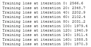

Recommendations

We will compute the ratings for all the movies and users and display the movies that are recommended.

These are based on the movies and ratings entered as my_ratings[]
To predict the rating of movie i for users j, we compute w⁽ⁱ⁾ * x⁽ⁱ⁾ + b⁽ⁱ⁾
This can be computed for all ratings using matrix multiplication

# Make a prediction using trained weights and biases
p = np.matmul(X.numpy(), np.transpose(W.numpy())) + b.numpy()

#restore the mean
pm = p + Ymean

my_predictions = pm[:,0]

# sort predictions
ix = tf.argsort(my_predictions, direction='DESCENDING')

for i in range(17):
    j = ix[i]
    if j not in my_rated:
        print(f'Predicting rating {my_predictions[j]:0.2f} for movie {movieList[j]}')

print('\n\nOriginal vs Predicted ratings:\n')
for i in range(len(my_ratings)):
    if my_ratings[i] > 0:
        print(f'Original {my_ratings[i]}, Predicted {my_predictions[i]:0.2f} for {movieList[i]}')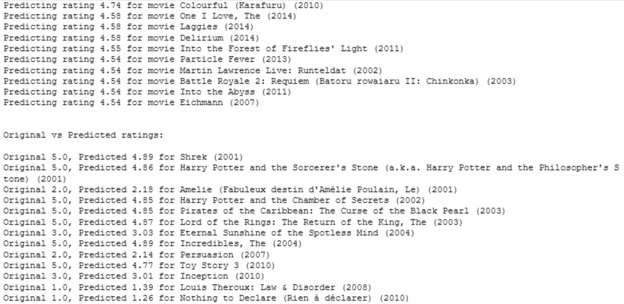

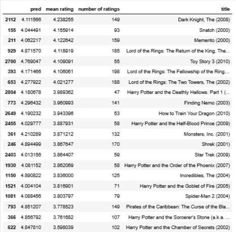
Additional information can be utilized to enhance our predictions.

Above, the predicted ratings for the first few hundred movies lie in a small range.
We can augment the above by selecting from those top movies, movies that have high average ratings and movies with more than 20 ratings.
This section uses a Pandas data frame which has many handy sorting features.

filter=(movieList_df["number of ratings"] > 20)
movieList_df["pred"] = my_predictions
movieList_df = movieList_df.reindex(columns=["pred", "mean rating", "number of ratings", "title"])
movieList_df.loc[ix[:300]].loc[filter].sort_values("mean rating", ascending=False)

Recommend Movies