Tips and Steps

Polynomial Regression

Setup

import numpy as np
%matplotlib widget
import matplotlib.pyplot as plt
from sklearn.linear_model import LinearRegression, Ridge
from sklearn.preprocessing import StandardScaler, PolynomialFeatures
from sklearn.model_selection import train_test_split
from sklearn.metrics import mean_squared_error
import tensorflow as tf
from tensorflow.keras.models import Sequential
from tensorflow.keras.layers import Dense
from tensorflow.keras.activations import relu,linear
from tensorflow.keras.losses import SparseCategoricalCrossentropy
from tensorflow.keras.optimizers import Adam

import logging
logging.getLogger("tensorflow").setLevel(logging.ERROR)

from public_tests_a1 import * 

tf.keras.backend.set_floatx('float64')
from assigment_utils import *

tf.autograph.set_verbosity(0)

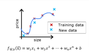
Let’s say you have created a machine learning model and you find it fits your training data very well. You’re done? Not quite. The goal of creating the model was to be able to predict values for new examples.

How can you test your model’s performance on new data before deploying it?
The answer has two parts:

Split your original data set into “Training” and “Test” sets.
- Use the training data to fit the parameters of the model
- Use the test data to evaluate the model on new data
Develop an error function to evaluate your model.

Split Data

Let’s use an sklearn function train_test_split to perform the split. Double-check the shapes after running the following cell.

# Generate some data
X,y,x_ideal,y_ideal = gen_data(18, 2, 0.7)
print("X.shape", X.shape, "y.shape", y.shape)

#split the data using sklearn routine 
X_train, X_test, y_train, y_test = train_test_split(X,y,test_size=0.33, random_state=1)
print("X_train.shape", X_train.shape, "y_train.shape", y_train.shape)
print("X_test.shape", X_test.shape, "y_test.shape", y_test.shape)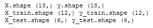

Plot

You can see below the data points that will be part of training (in red) are intermixed with those that the model is not trained on (test). This particular data set is a quadratic function with noise added. The “ideal” curve is shown for reference.

fig, ax = plt.subplots(1,1,figsize=(4,4))
ax.plot(x_ideal, y_ideal, "--", color = "orangered", label="y_ideal", lw=1)
ax.set_title("Training, Test",fontsize = 14)
ax.set_xlabel("x")
ax.set_ylabel("y")

ax.scatter(X_train, y_train, color = "red",           label="train")
ax.scatter(X_test, y_test,   color = dlc["dlblue"],   label="test")
ax.legend(loc='upper left')
plt.show()

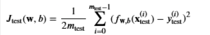
MSE Calculation

When evaluating a linear regression model, you average the squared error difference of the predicted values and the target values.

def eval_mse(y, yhat):
    """ 
    Calculate the mean squared error on a data set.
    Args:
      y    : (ndarray  Shape (m,) or (m,1))  target value of each example
      yhat : (ndarray  Shape (m,) or (m,1))  predicted value of each example
    Returns:
      err: (scalar)             
    """
    m = len(y)
    err = 0.0
    for i in range(m):
        err_i = (yhat[i] - y[i])**2   
        err += err_i
    err = err / (2*m)
    
    return(err)

Compare Train vs Test

Let’s build a high degree polynomial model to minimize training error. This will use the linear_regression functions from sklearn. The code is in the imported utility file if you would like to see the details. The steps below are:

create and fit the model. (‘fit’ is another name for training or running gradient descent).
compute the error on the training data.
compute the error on the test data.

# create a model in sklearn, train on training data
degree = 10
lmodel = lin_model(degree)
lmodel.fit(X_train, y_train)

# predict on training data, find training error
yhat = lmodel.predict(X_train)
err_train = lmodel.mse(y_train, yhat)

# predict on test data, find error
yhat = lmodel.predict(X_test)
err_test = lmodel.mse(y_test, yhat)

print(f"training err {err_train:0.2f}, test err {err_test:0.2f}")

The computed error on the training set is substantially less than that of the test set, look at the plot below for the reason why

# plot predictions over data range 
x = np.linspace(0,int(X.max()),100)  # predict values for plot
y_pred = lmodel.predict(x).reshape(-1,1)

plt_train_test(X_train, y_train, X_test, y_test, x, y_pred, x_ideal, y_ideal, degree)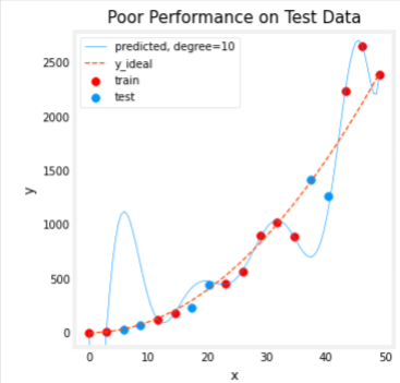

The test set error shows this model will not work well on new data. If you use the test error to guide improvements in the model, then the model will perform well on the test data… but the test data was meant to represent new data. You need yet another set of data to test new data performance.

The proposal made during lecture is to separate data into three groups. The distribution of training, cross-validation and test sets shown in the below table is a typical distribution, but can be varied depending on the amount of data available.

data	% of total	Description
training	60	Data used to tune model parameters 𝑤w and 𝑏b in training or fitting
cross-validation	20	Data used to tune other model parameters like degree of polynomial, regularization or the architecture of a neural network.
test	20	Data used to test the model after tuning to gauge performance on new data

3 Split

Let’s generate three data sets below. We’ll once again use train_test_split from sklearn but will call it twice to get three splits:

# Generate  data
X,y, x_ideal,y_ideal = gen_data(40, 5, 0.7)
print("X.shape", X.shape, "y.shape", y.shape)

#split the data using sklearn routine 
X_train, X_, y_train, y_ = train_test_split(X,y,test_size=0.40, random_state=1)
X_cv, X_test, y_cv, y_test = train_test_split(X_,y_,test_size=0.50, random_state=1)
print("X_train.shape", X_train.shape, "y_train.shape", y_train.shape)
print("X_cv.shape", X_cv.shape, "y_cv.shape", y_cv.shape)
print("X_test.shape", X_test.shape, "y_test.shape", y_test.shape)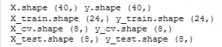

Bias & Variance

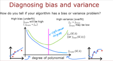
Above, it was clear the degree of the polynomial model was too high. How can you choose a good value? It turns out, as shown in the diagram, the training and cross-validation performance can provide guidance. By trying a range of degree values, the training and cross-validation performance can be evaluated. As the degree becomes too large, the cross-validation performance will start to degrade relative to the training performance. Let’s try this on our example.

Plot All 3

fig, ax = plt.subplots(1,1,figsize=(4,4))
ax.plot(x_ideal, y_ideal, "--", color = "orangered", label="y_ideal", lw=1)
ax.set_title("Training, CV, Test",fontsize = 14)
ax.set_xlabel("x")
ax.set_ylabel("y")

ax.scatter(X_train, y_train, color = "red",           label="train")
ax.scatter(X_cv, y_cv,       color = dlc["dlorange"], label="cv")
ax.scatter(X_test, y_test,   color = dlc["dlblue"],   label="test")
ax.legend(loc='upper left')
plt.show()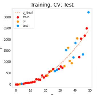

Train the model repeatedly, increasing the degree of the polynomial each iteration. We’re going to use the scikit-learn linear regression model for speed and simplicity

max_degree = 9
err_train = np.zeros(max_degree)    
err_cv = np.zeros(max_degree)      
x = np.linspace(0,int(X.max()),100)  
y_pred = np.zeros((100,max_degree))  #columns are lines to plot

for degree in range(max_degree):
    lmodel = lin_model(degree+1)
    lmodel.fit(X_train, y_train)
    yhat = lmodel.predict(X_train)
    err_train[degree] = lmodel.mse(y_train, yhat)
    yhat = lmodel.predict(X_cv)
    err_cv[degree] = lmodel.mse(y_cv, yhat)
    y_pred[:,degree] = lmodel.predict(x)
    
optimal_degree = np.argmin(err_cv)+1

plt.close("all")
plt_optimal_degree(X_train, y_train, X_cv, y_cv, x, y_pred, x_ideal, y_ideal, 
                   err_train, err_cv, optimal_degree, max_degree)

The plot above demonstrates that separating data into two groups, data the model is trained on and data the model has not been trained on, can be used to determine if the model is underfitting or overfitting. In our example, we created a variety of models varying from underfitting to overfitting by increasing the degree of the polynomial used.

On the left plot, the solid lines represent the predictions from these models. A polynomial model with degree 1 produces a straight line that intersects very few data points, while the maximum degree hews very closely to every data point.
on the right:
- the error on the trained data (blue) decreases as the model complexity increases as expected
- the error of the cross-validation data decreases initially as the model starts to conform to the data, but then increases as the model starts to over-fit on the training data (fails to generalize).

It’s worth noting that the curves in these examples as not as smooth as one might draw for a lecture. It’s clear the specific data points assigned to each group can change your results significantly. The general trend is what is important.

Regularization

We have utilized regularization to reduce overfitting. Similar to degree, one can use the same methodology to tune the regularization parameter lambda (𝜆λ).

Let’s demonstrate this by starting with a high degree polynomial and varying the regularization parameter.

lambda_range = np.array([0.0, 1e-6, 1e-5, 1e-4,1e-3,1e-2, 1e-1,1,10,100])
num_steps = len(lambda_range)
degree = 10
err_train = np.zeros(num_steps)    
err_cv = np.zeros(num_steps)       
x = np.linspace(0,int(X.max()),100) 
y_pred = np.zeros((100,num_steps))  #columns are lines to plot

for i in range(num_steps):
    lambda_= lambda_range[i]
    lmodel = lin_model(degree, regularization=True, lambda_=lambda_)
    lmodel.fit(X_train, y_train)
    yhat = lmodel.predict(X_train)
    err_train[i] = lmodel.mse(y_train, yhat)
    yhat = lmodel.predict(X_cv)
    err_cv[i] = lmodel.mse(y_cv, yhat)
    y_pred[:,i] = lmodel.predict(x)
    
optimal_reg_idx = np.argmin(err_cv)

plt.close("all")
plt_tune_regularization(X_train, y_train, X_cv, y_cv, x, y_pred, err_train, err_cv, optimal_reg_idx, lambda_range)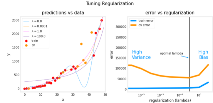

The plots show that as regularization increases, the model moves from a high variance (overfitting) model to a high bias (underfitting) model. The vertical line in the right plot shows the optimal value of lambda. In this example, the polynomial degree was set to 10.

Increase Data Size

m is the size of the data set

X_train, y_train, X_cv, y_cv, x, y_pred, err_train, err_cv, m_range,degree = tune_m()
plt_tune_m(X_train, y_train, X_cv, y_cv, x, y_pred, err_train, err_cv, m_range, degree)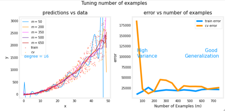

The above plots show that when a model has high variance and is overfitting, adding more examples improves performance. Note the curves on the left plot. The final curve with the highest value of 𝑚m is a smooth curve that is in the center of the data. On the right, as the number of examples increases, the performance of the training set and cross-validation set converge to similar values. Note that the curves are not as smooth as one might see in a lecture. That is to be expected. The trend remains clear: more data improves generalization.

Note that adding more examples when the model has high bias (underfitting) does not improve performance.

Evaluating NN

# Generate and split data set
X, y, centers, classes, std = gen_blobs()

# split the data. Large CV population for demonstration
X_train, X_, y_train, y_ = train_test_split(X,y,test_size=0.50, random_state=1)
X_cv, X_test, y_cv, y_test = train_test_split(X_,y_,test_size=0.20, random_state=1)
print("X_train.shape:", X_train.shape, "X_cv.shape:", X_cv.shape, "X_test.shape:", X_test.shape)

plt_train_eq_dist(X_train, y_train,classes, X_cv, y_cv, centers, std)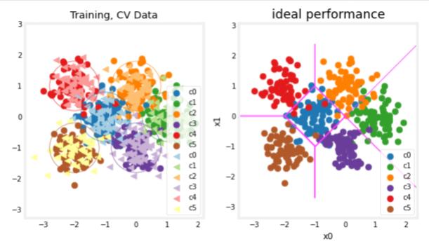

Above, you can see the data on the left. There are six clusters identified by color. Both training points (dots) and cross-validataion points (triangles) are shown. The interesting points are those that fall in ambiguous locations where either cluster might consider them members. What would you expect a neural network model to do? What would be an example of overfitting? underfitting?
On the right is an example of an ‘ideal’ model, or a model one might create knowing the source of the data. The lines represent ‘equal distance’ boundaries where the distance between center points is equal. It’s worth noting that this model would “misclassify” roughly 8% of the total data set.

Error Calculation

For categorical models, we simply find the fraction of incorrect predictions

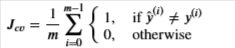
def eval_cat_err(y, yhat):
    """ 
    Calculate the categorization error
    Args:
      y    : (ndarray  Shape (m,) or (m,1))  target value of each example
      yhat : (ndarray  Shape (m,) or (m,1))  predicted value of each example
    Returns:|
      cerr: (scalar)             
    """
    m = len(y)
    incorrect = 0
    for i in range(m):
       if yhat[i] != y[i]:
            incorrect += 1
    cerr = incorrect/m 
    
    return(cerr)

y_hat = np.array([1, 2, 0])
y_tmp = np.array([1, 2, 3])
print(f"categorization error {np.squeeze(eval_cat_err(y_hat, y_tmp)):0.3f}, expected:0.333" )
y_hat = np.array([[1], [2], [0], [3]])
y_tmp = np.array([[1], [2], [1], [3]])
print(f"categorization error {np.squeeze(eval_cat_err(y_hat, y_tmp)):0.3f}, expected:0.250" )

 
test_eval_cat_er

Model Complexity

We will build two models, one simple and one more complex. We will then evaluate the models to determine if the are likely to overfit or underfit

Complex Model

Compose a three-layer model:

Dense layer with 120 units, relu activation
Dense layer with 40 units, relu activation
Dense layer with 6 units and a linear activation (not softmax)
Compile using
loss with SparseCategoricalCrossentropy, remember to use from_logits=True
Adam optimizer with learning rate of 0.01.

import logging
logging.getLogger("tensorflow").setLevel(logging.ERROR)

tf.random.set_seed(1234)
model = Sequential(
    [
        Dense(units=120, activation='relu', name="L1"),
        Dense(units=40, activation='relu', name="L2"),
        Dense(units=6, activation='linear', name="L3")
    ], name="Complex"
)
model.compile(
    loss=tf.keras.losses.SparseCategoricalCrossentropy(from_logits=True),
    optimizer=tf.keras.optimizers.Adam(0.01),
)

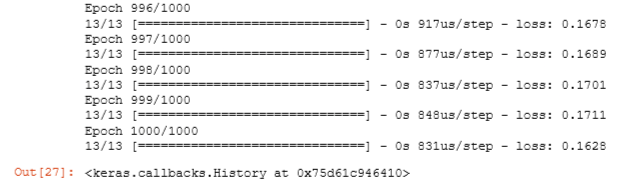
model.fit(
    X_train, y_train,
    epochs=1000
)

model.summary()

model_test(model, classes, X_train.shape[1])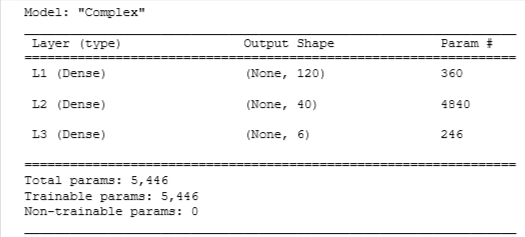

Plot

#make a model for plotting routines to call
model_predict = lambda Xl: np.argmax(tf.nn.softmax(model.predict(Xl)).numpy(),axis=1)
plt_nn(model_predict,X_train,y_train, classes, X_cv, y_cv, suptitle="Complex Model")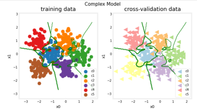

This model has worked very hard to capture outliers of each category. As a result, it has miscategorized some of the cross-validation data. Let’s calculate the classification error.

Error

training_cerr_complex = eval_cat_err(y_train, model_predict(X_train))
cv_cerr_complex = eval_cat_err(y_cv, model_predict(X_cv))
print(f"categorization error, training, complex model: {training_cerr_complex:0.3f}")
print(f"categorization error, cv,       complex model: {cv_cerr_complex:0.3f}")

Simple Model

Dense layer with 6 units, relu activation
Dense layer with 6 units and a linear activation. Compile using
loss with SparseCategoricalCrossentropy, remember to use from_logits=True
Adam optimizer with learning rate of 0.01.

tf.random.set_seed(1234)
model_s = Sequential(
    [
        Dense(6, activation = 'relu', name="L1"), 
        Dense(classes, activation = 'linear', name="L2")        
    ], name = "Simple"
)
model_s.compile(
    loss=tf.keras.losses.SparseCategoricalCrossentropy(from_logits=True), 
    optimizer=tf.keras.optimizers.Adam(0.01),
)

import logging
logging.getLogger("tensorflow").setLevel(logging.ERROR)

model_s.fit(
    X_train,y_train,
    epochs=1000
)

model_s.summary()

model_s_test(model_s, classes, X_train.shape[1])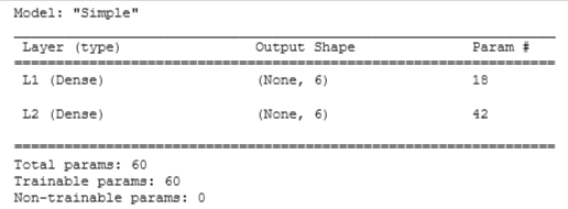

Plot

#make a model for plotting routines to call
model_predict_s = lambda Xl: np.argmax(tf.nn.softmax(model_s.predict(Xl)).numpy(),axis=1)
plt_nn(model_predict_s,X_train,y_train, classes, X_cv, y_cv, suptitle="Simple Model")

Error Calculation

training_cerr_simple = eval_cat_err(y_train, model_predict_s(X_train))
cv_cerr_simple = eval_cat_err(y_cv, model_predict_s(X_cv))
print(f"categorization error, training, simple model, {training_cerr_simple:0.3f}, complex model: {training_cerr_complex:0.3f}" )
print(f"categorization error, cv,       simple model, {cv_cerr_simple:0.3f}, complex model: {cv_cerr_complex:0.3f}"

Our simple model has a little higher classification error on training data but does better on cross-validation data than the more complex model.

Regularization

Reconstruct your complex model, but this time include regularization. Below, compose a three-layer model:

Dense layer with 120 units, relu activation, kernel_regularizer=tf.keras.regularizers.l2(0.1)
Dense layer with 40 units, relu activation, kernel_regularizer=tf.keras.regularizers.l2(0.1)
Dense layer with 6 units and a linear activation. Compile using
loss with SparseCategoricalCrossentropy, remember to use from_logits=True
Adam optimizer with learning rate of 0.01.

tf.random.set_seed(1234)
model_r = Sequential(
    [
        Dense(120, activation = 'relu', kernel_regularizer=tf.keras.regularizers.l2(0.1), name="L1"), 
        Dense(40, activation = 'relu', kernel_regularizer=tf.keras.regularizers.l2(0.1), name="L2"),  
        Dense(classes, activation = 'linear', name="L3")  
    ], name="ComplexRegularized"
)
model_r.compile(
        loss=tf.keras.losses.SparseCategoricalCrossentropy(from_logits=True), 
        optimizer=tf.keras.optimizers.Adam(0.01), 
)

model_r.fit(
    X_train, y_train,
    epochs=1000
)

model_r.summary()

model_r_test(model_r, classes, X_train.shape[1])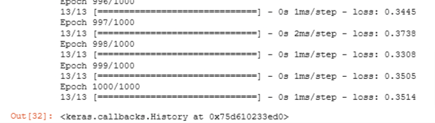

#make a model for plotting routines to call
model_predict_r = lambda Xl: np.argmax(tf.nn.softmax(model_r.predict(Xl)).numpy(),axis=1)
 
plt_nn(model_predict_r, X_train,y_train, classes, X_cv, y_cv, suptitle="Regularized")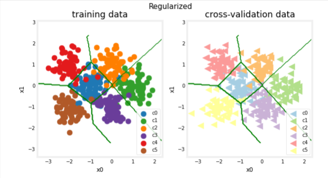

training_cerr_reg = eval_cat_err(y_train, model_predict_r(X_train))
cv_cerr_reg = eval_cat_err(y_cv, model_predict_r(X_cv))
test_cerr_reg = eval_cat_err(y_test, model_predict_r(X_test))
print(f"categorization error, training, regularized: {training_cerr_reg:0.3f}, simple model, {training_cerr_simple:0.3f}, complex model: {training_cerr_complex:0.3f}" )
print(f"categorization error, cv,       regularized: {cv_cerr_reg:0.3f}, simple model, {cv_cerr_simple:0.3f}, complex model: {cv_cerr_complex:0.3f}" )

Optimal Regularization Value

As we did in linear regression, you can try many regularization values. This code takes several minutes to run. If you have time, you can run it and check the results. If not, you have completed the graded parts of the assignment!

tf.random.set_seed(1234)
lambdas = [0.0, 0.001, 0.01, 0.05, 0.1, 0.2, 0.3]
models=[None] * len(lambdas)

for i in range(len(lambdas)):
    lambda_ = lambdas[i]
    models[i] =  Sequential(
        [
            Dense(120, activation = 'relu', kernel_regularizer=tf.keras.regularizers.l2(lambda_)),
            Dense(40, activation = 'relu', kernel_regularizer=tf.keras.regularizers.l2(lambda_)),
            Dense(classes, activation = 'linear')
        ]
    )
    models[i].compile(
        loss=tf.keras.losses.SparseCategoricalCrossentropy(from_logits=True),
        optimizer=tf.keras.optimizers.Adam(0.01),
    )

    models[i].fit(
        X_train,y_train,
        epochs=1000
    )
    print(f"Finished lambda = {lambda_}")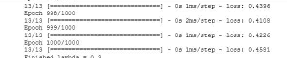

plot_iterate(lambdas, models, X_train, y_train, X_cv, y_cv)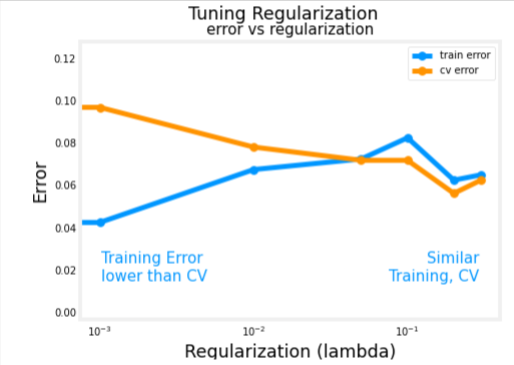

Let’s test the optimized models and compare them to the ideal performance

plt_compare(X_test,y_test, classes, model_predict_s, model_predict_r, centers)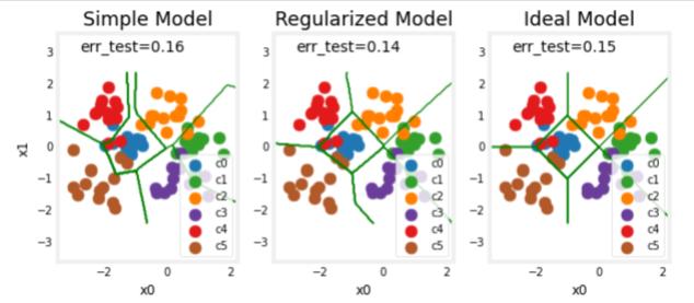

Our test set is small and seems to have a number of outliers so classification error is high. However, the performance of our optimized models is comparable to ideal performance.