Cost Function

My thanks and credit to Stanford University & Andrew Ng for their contributions.

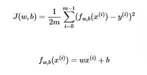
If you recall the cost function for a single variable is along with the LR formula:

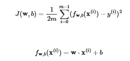
Not much changes for multivariables except that w and x⁽ⁱ⁾ are vectors supporting multiple features, and not scalars like they were earlier

Code

---

Setup

import copy, math
import numpy as np
import matplotlib.pyplot as plt
plt.style.use('./deeplearning.mplstyle')
np.set_printoptions(precision=2)  # reduced display precision on numpy arrays

.

Data

X_train = np.array([[2104, 5, 1, 45], [1416, 3, 2, 40], [852, 2, 1, 35]])
y_train = np.array([460, 232, 178])

# data is stored in numpy array/matrix
print(f"X Shape: {X_train.shape}, X Type:{type(X_train)})")
print(X_train)
print(f"y Shape: {y_train.shape}, y Type:{type(y_train)})")
print(y_train)

X Shape: (3, 4), X Type:<class 'numpy.ndarray'>)
[[2104    5    1   45]
 [1416    3    2   40]
 [ 852    2    1   35]]
y Shape: (3,), y Type:<class 'numpy.ndarray'>)
[460 232 178]

# set initial values for b & w
b_init = 785.1811367994083
w_init = np.array([ 0.39133535, 18.75376741, -53.36032453, -26.42131618])
print(f"w_init shape: {w_init.shape}, b_init type: {type(b_init)}")

w_init shape: (4,), b_init type: <class 'float'>

Cost

def compute_cost(X, y, w, b): 
    """
    compute cost
    Args:
      X (ndarray (m,n)): Data, m examples with n features
      y (ndarray (m,)) : target values
      w (ndarray (n,)) : model parameters  
      b (scalar)       : model parameter
      
    Returns:
      cost (scalar): cost
    """
    m = X.shape[0]
    cost = 0.0
    for i in range(m):                                
        f_wb_i = np.dot(X[i], w) + b           #(n,)(n,) = scalar (see np.dot)
        cost = cost + (f_wb_i - y[i])**2       #scalar
    cost = cost / (2 * m)                      #scalar    
    return cost

# Compute and display cost using our pre-chosen optimal parameters. 
cost = compute_cost(X_train, y_train, w_init, b_init)
print(f'Cost at optimal w : {cost}')

Cost at optimal w : 1.5578904428966628e-12