import math, copy
import numpy as np
import matplotlib.pyplot as plt
plt.style.use('./deeplearning.mplstyle')
from lab_utils_uni import plt_house_x, plt_contour_wgrad, plt_divergence, plt_gradients

# Load our data set
x_train = np.array([1.0, 2.0])   #features
y_train = np.array([300.0, 500.0]) #target valueGradient Descent
My thanks and credit to Stanford University & Andrew Ng for their contributions.
An algorithm to find the minimum cost value of not only linear regression models but deep learning models as well. The purpose is to minimize the cost function, as it turns out it is very useful to minimize ANY function
It will give you the value that will minimize the cost of any function by providing the values of w & b regardless of how many parameters there are.
Recap
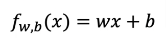
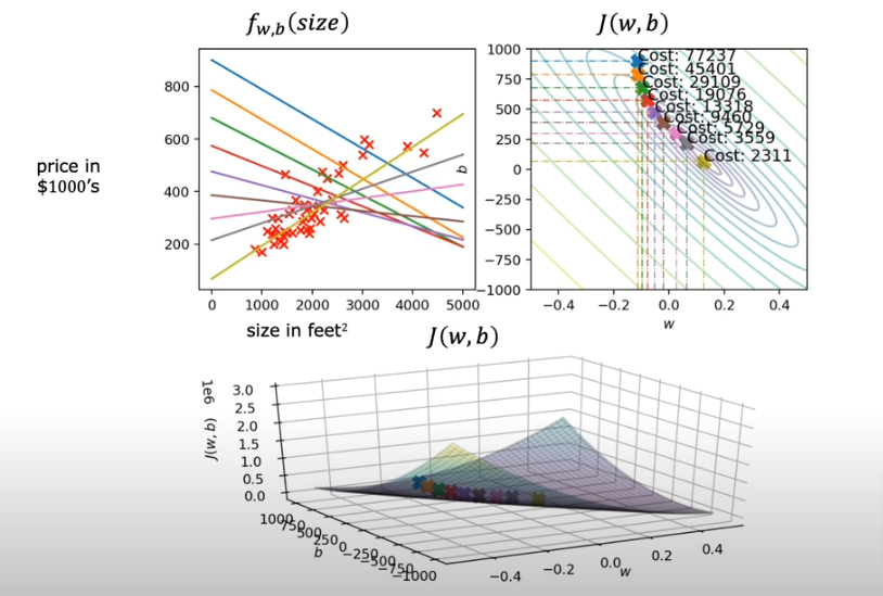
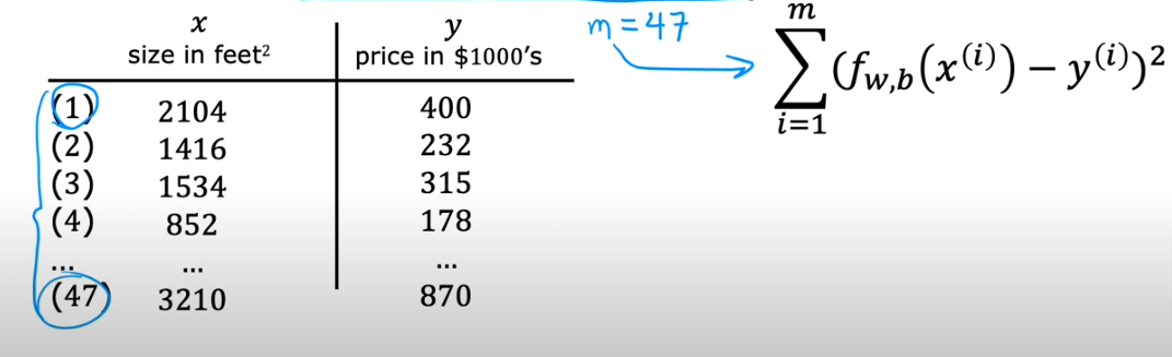
Remember the linear model we worked on the past two pages:
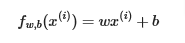
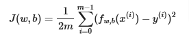
In linear regression, you utilize input training data to fit the parameters w,b by minimizing a measure of the error between our predictions fw,b(x(i)) and the actual data y(i). The measure is called the cost, J(w,b). In training you measure the cost over all of our training samples
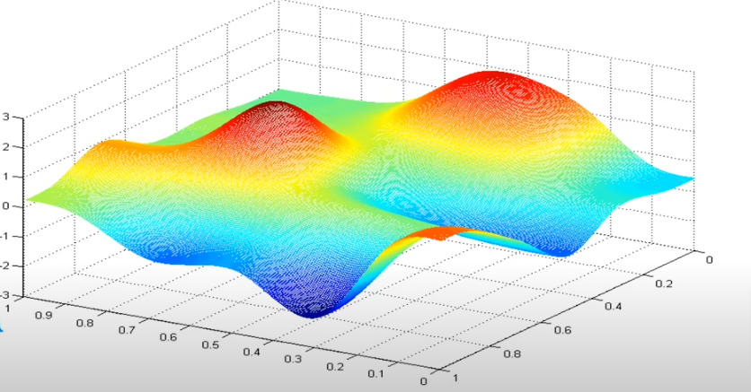
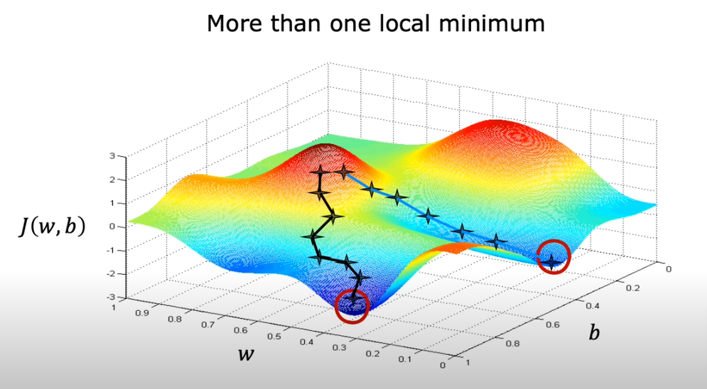
The bow/hammock shape we got earlier is an indication of a regression model, but for neural networks we get a bubble shape like this below. You basically imagine yourself on top of one of the hills (dark red) and you want to make your way down to the lowest value (dark blue), if you move your starting point by one or two steps in any direction and travel down the easiest way it will most likely land you at a completely different lowest point than the previous one.
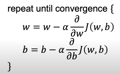
- So starting by choosing w, and the next time you choose a small variation away from w to start your descent
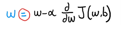
- Here we are assigning the new variance to w after we adjust w by (-alpha…..)
- alpha = learning rate, a number very close to zero, it is the size of the steps we are taking downhill, so we want to take smallest steps
- the learning rate is always positive. The d/dw is the slope of J(w,b) so as the slope gets closer to closer to zero we know we are getting closer to the minimum value.
- what’s after alpha is a derivative of function J which is the direction we want to take from the top of the hill
- we also assign a new value for b as well
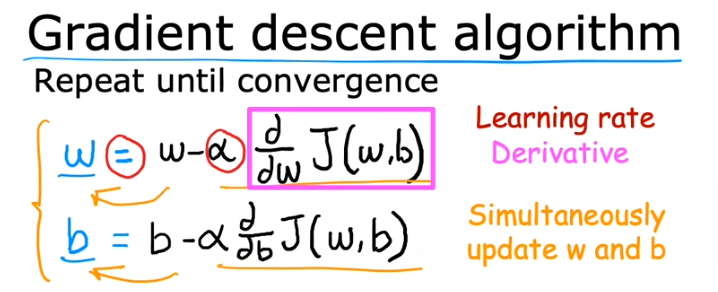
- so just as we did take baby steps when we chose w and started the descent downhill, we do the same for b, we take small variance from b and take small steps and we keep repeating the descent for both w & b until we find a convergence
- Convergence happens when we reach the local minimum and neither w nor b change much after the next step, that’s when we know we are there
- One very important point is: you need to update the small variance for both b & w simultaneously. So notice that in the correct version, w used in the first line if the pre-updated w and it is the same pre-updated value that does into tmp_b as well.
- While looking at the incorrect way, the w used in tmp_b has already been updated and therefore incorrect because tmp_w has not been updated yet and that’s not being done simultaneously
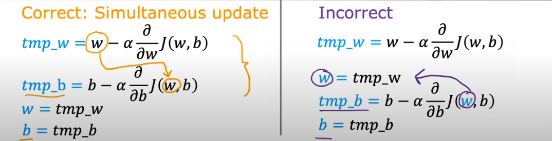
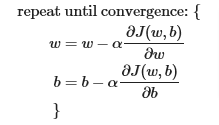
- So in summary, the gradient descent is described as code below where parameters w and b are updated simultaneously
ALPHA - learning rate
In the same way if we choose a large number for the learning rate we end up overshooting the minimum value and never converge.
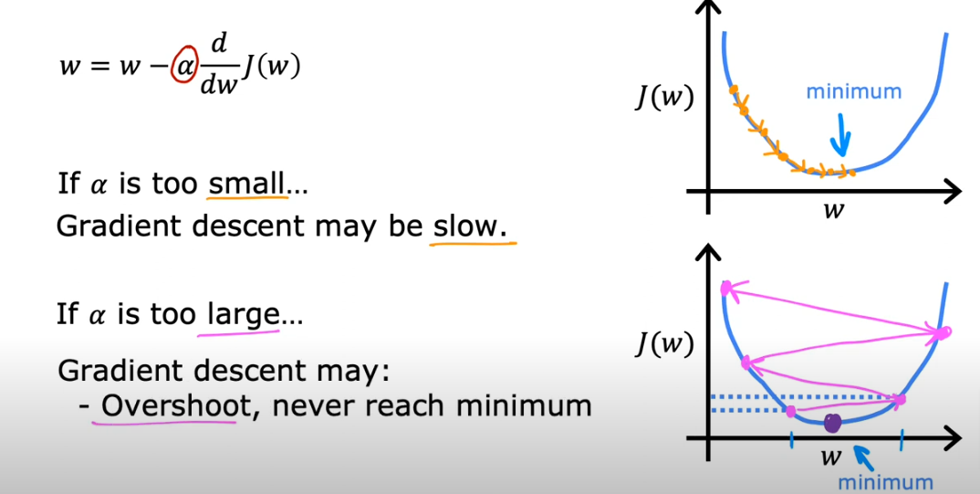
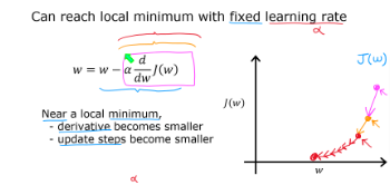
What if we don’t have a square error cost function (which is just one concave line (bowl shape)) as shown in the image above, but we have a curve with multiple peaks and local minimums, as you see above at the start of this page.
The question is: what does the gradient descent do if we already reached one of the minimums?
What we have to understand is even if we don’t vary \({\alpha}\) gradient descent will know slow down as we get closer to the minimum. Reason being is the derivative (which is the slope of J() at the point on the curve will decrease as the points get closer to the bottom/minimum so as the slope gets smaller the product of the formula will automatically get smaller even if we don’t lower the value of \({\alpha}\)
That’s why the gradient descent can reach a minimum with a fixed valued of \({\alpha}\)

GD for Linear Regression Model
So now let’s put the Gradient Descent & Cost Formula together to train a Linear Regression Model to best fit the line
So let’s bring them all together here:
Linear Regression Model
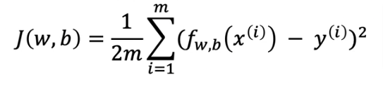
Cost Function
From earlier this is the same cost function from the previous page and we will use the function compute_cost in the code section below just as we did in previous section
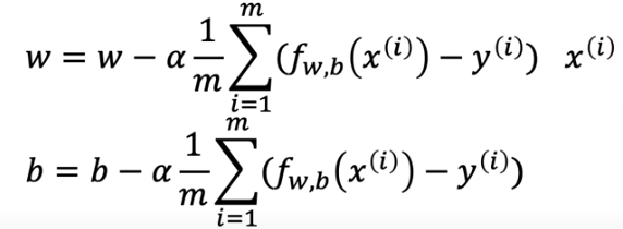
Gradient Descent Algorithm
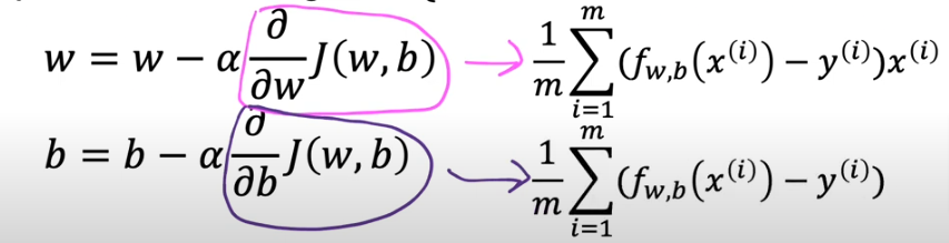
To break down the algorithm you will see that the math of the derivative will yield equations 4 & 5 on the right side below. In the code section below we will use compute_gradient to calculate them
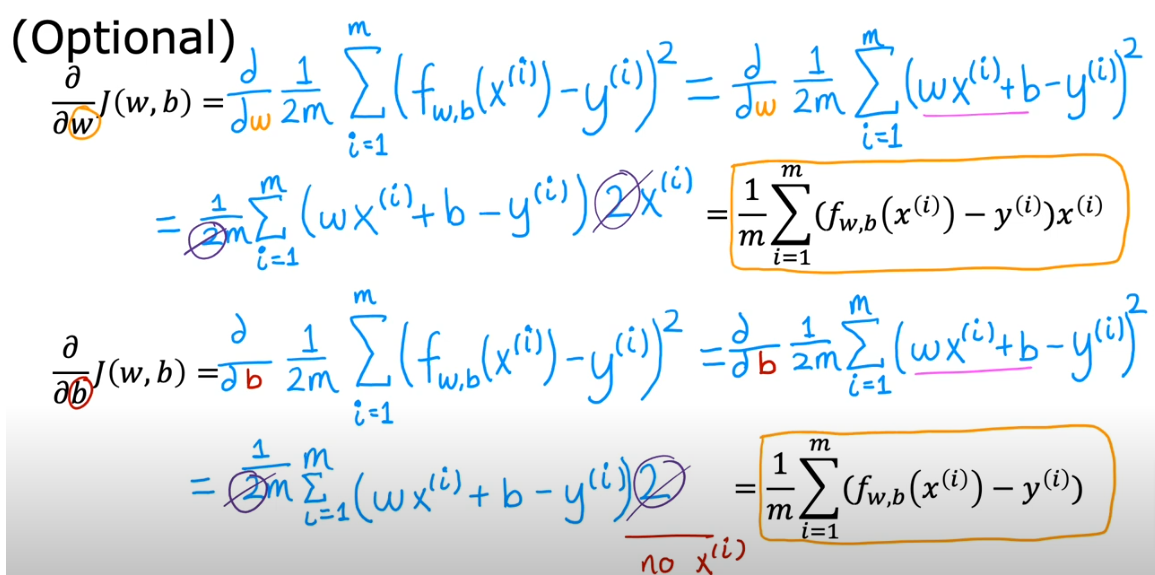
Calculus
If you go through the calculus of the derivatives you’ll see this is how we arrived at the formula above
GD Algorithm
combined together will give us gradient descent which will be shown in the function gradient_descent in the code section below ( utilizes both compute_gradient and compute_cost)
- The first line shows the derivative of the cost function with respect to w (what follows \({\alpha}\))
- The second line shows the derivative of the cost function with respect to b
- Reminder: we have to update w and b simultaneously
- Remember for multiple local minimums that you can end up at different local minimums depending on where you initialize the initial position of w & b
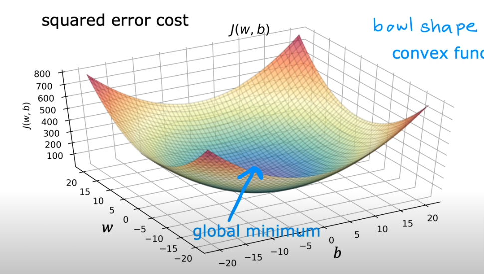
- And with squared error cost function the function will ALWAYS have ONE local minimum, it is called convex function also. The local minimum is also know as global minimum
How To Use
- So let’s start with our linear regression model we started a few pages ago and assign w=-0.1 b=900
- Then we take one step from the blue to orange and you see the line has changed
- Take more steps towards the middle and you see the straight line fit till we reach the global minimum shown below using the mustard colored line
Batch Gradient Descent
So if we use the algorithm above to arrive at the mustard line based on the housing prices in the dataset, we in essence use all the training sets in the data and therefore it is called Batch gradient descent Not a subset of the data.
Other models will use subsets of data, but we will use the entire dataset for linear regression models
Code
.
Compute Cost
#Function to calculate the cost
def compute_cost(x, y, w, b):

    m = x.shape[0]
    cost = 0

    for i in range(m):
        f_wb = w * x[i] + b
        cost = cost + (f_wb - y[i])**2
    total_cost = 1 / (2 * m) * cost

    return total_cost
Compute Gradient
def compute_gradient(x, y, w, b):
    """
    Computes the gradient for linear regression
    Args:
      x (ndarray (m,)): Data, m examples
      y (ndarray (m,)): target values
      w,b (scalar)    : model parameters
    Returns
      dj_dw (scalar): The gradient of the cost w.r.t. (with respect to) the parameters w
      dj_db (scalar): The gradient of the cost w.r.t. the parameter b
     """

    # Number of training examples
    m = x.shape[0]
    dj_dw = 0
    dj_db = 0

    for i in range(m):
        f_wb = w * x[i] + b
        dj_dw_i = (f_wb - y[i]) * x[i]
        dj_db_i = f_wb - y[i]
        dj_db += dj_db_i
        dj_dw += dj_dw_i
    dj_dw = dj_dw / m
    dj_db = dj_db / m

    return dj_dw, dj_db
plt_gradients(x_train,y_train, compute_cost, compute_gradient)
plt.show()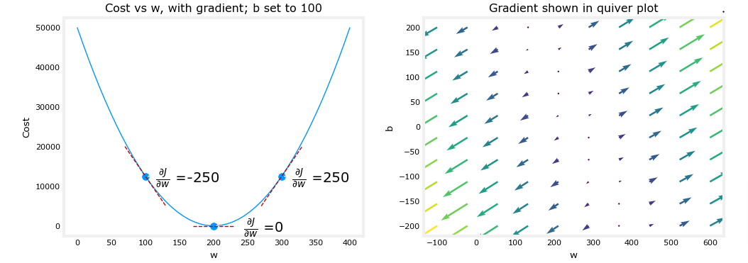
Above, the left plot shows ∂J(w,b)∂w or the slope of the cost curve relative to w at three points. On the right side of the plot, the derivative is positive, while on the left it is negative. Due to the ‘bowl shape’, the derivatives will always lead gradient descent toward the bottom where the gradient is zero.
The left plot has fixed b=100. Gradient descent will utilize both ∂J(w,b)∂w and ∂J(w,b)∂b to update parameters. The ‘quiver plot’ on the right provides a means of viewing the gradient of both parameters. The arrow sizes reflect the magnitude of the gradient at that point. The direction and slope of the arrow reflects the ratio of ∂J(w,b)∂w and ∂J(w,b)∂b at that point. Note that the gradient points away from the minimum. Review equation (3) above. The scaled gradient is subtracted from the current value of w or b. This moves the parameter in a direction that will reduce cost.
Gradient Descent
def gradient_descent(x, y, w_in, b_in, alpha, num_iters, cost_function, gradient_function):
    """
    Performs gradient descent to fit w,b. Updates w,b by taking
    num_iters gradient steps with learning rate alpha

    Args:
      x (ndarray (m,))  : Data, m examples
      y (ndarray (m,))  : target values
      w_in,b_in (scalar): initial values of model parameters
      alpha (float):     Learning rate
      num_iters (int):   number of iterations to run gradient descent
      cost_function:     function to call to produce cost
      gradient_function: function to call to produce gradient

    Returns:
      w (scalar): Updated value of parameter after running gradient descent
      b (scalar): Updated value of parameter after running gradient descent
      J_history (List): History of cost values
      p_history (list): History of parameters [w,b]
      """

    w = copy.deepcopy(w_in) # avoid modifying global w_in
    # An array to store cost J and w's at each iteration primarily for graphing later
    J_history = []
    p_history = []
    b = b_in
    w = w_in

    for i in range(num_iters):
        # Calculate the gradient and update the parameters using gradient_function
        dj_dw, dj_db = gradient_function(x, y, w , b)

        # Update Parameters using equation (3) above
        b = b - alpha * dj_db
        w = w - alpha * dj_dw

        # Save cost J at each iteration
        if i<100000:      # prevent resource exhaustion
            J_history.append( cost_function(x, y, w , b))
            p_history.append([w,b])
        # Print cost every at intervals 10 times or as many iterations if < 10
        if i% math.ceil(num_iters/10) == 0:
            print(f"Iteration {i:4}: Cost {J_history[-1]:0.2e} ",
                  f"dj_dw: {dj_dw: 0.3e}, dj_db: {dj_db: 0.3e}  ",
                  f"w: {w: 0.3e}, b:{b: 0.5e}")

    return w, b, J_history, p_history #return w and J,w history for graphing
# initialize parameters
w_init = 0
b_init = 0
# some gradient descent settings
iterations = 10000
tmp_alpha = 1.0e-2
# run gradient descent
w_final, b_final, J_hist, p_hist = gradient_descent(x_train ,y_train, w_init, b_init, tmp_alpha,
iterations, compute_cost, compute_gradient)
print(f"(w,b) found by gradient descent: ({w_final:8.4f},{b_final:8.4f})")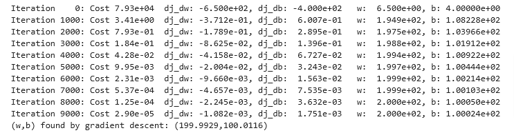
- The cost starts large and rapidly declines as described in the slide from the lecture.
- The partial derivatives,
dj_dw, anddj_dbalso get smaller, rapidly at first and then more slowly. As shown in the diagram from the lecture, as the process nears the ‘bottom of the bowl’ progress is slower due to the smaller value of the derivative at that point. - progress slows though the learning rate, alpha, remains fixed
Cost vs Iterations
A plot of cost versus iterations is a useful measure of progress in gradient descent. Cost should always decrease in successful runs. The change in cost is so rapid initially, it is useful to plot the initial decent on a different scale than the final descent. In the plots below, note the scale of cost on the axes and the iteration step.
# plot cost versus iteration
fig, (ax1, ax2) = plt.subplots(1, 2, constrained_layout=True, figsize=(12,4))
ax1.plot(J_hist[:100])
ax2.plot(1000 + np.arange(len(J_hist[1000:])), J_hist[1000:])
ax1.set_title("Cost vs. iteration(start)");  ax2.set_title("Cost vs. iteration (end)")
ax1.set_ylabel('Cost')            ;  ax2.set_ylabel('Cost')
ax1.set_xlabel('iteration step')  ;  ax2.set_xlabel('iteration step')
plt.show()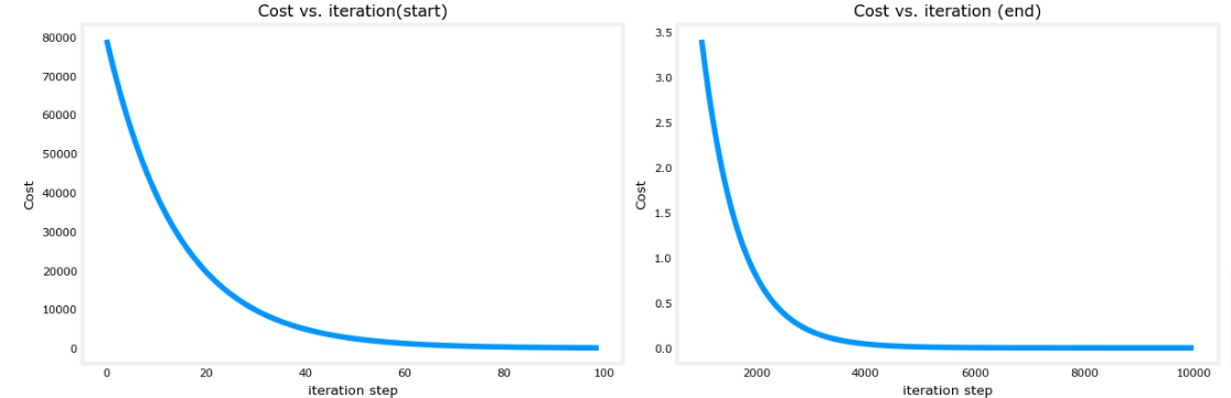
Now that we have found the optimal values for w and b we can predict the housing values.
print(f"1000 sqft house prediction {w_final*1.0 + b_final:0.1f} Thousand dollars")
print(f"1200 sqft house prediction {w_final*1.2 + b_final:0.1f} Thousand dollars")
print(f"2000 sqft house prediction {w_final*2.0 + b_final:0.1f} Thousand dollars")
1000 sqft house prediction 300.0 Thousand dollars 1200 sqft house prediction 340.0 Thousand dollars 2000 sqft house prediction 500.0 Thousand dollars
Contour Plot
- You can show the progress of gradient descent during its execution by plotting the cost over iterations on a contour plot of the cost(w,b).
fig, ax = plt.subplots(1,1, figsize=(12, 6))
plt_contour_wgrad(x_train, y_train, p_hist, ax)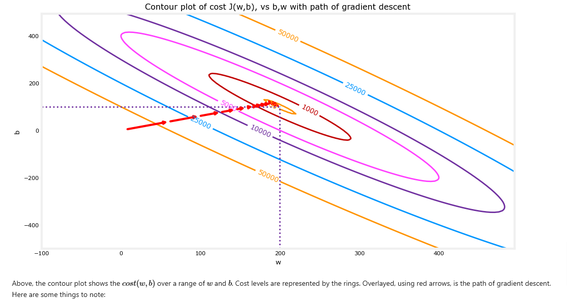
- The path makes steady (monotonic) progress toward its goal.
- initial steps are much larger than the steps near the goal.
- If we zoom in, the distance between steps shrinks and the gradient approaches zero
fig, ax = plt.subplots(1,1, figsize=(12, 4))
plt_contour_wgrad(x_train, y_train, p_hist, ax, w_range=[180, 220, 0.5], b_range=[80, 120, 0.5],
            contours=[1,5,10,20],resolution=0.5)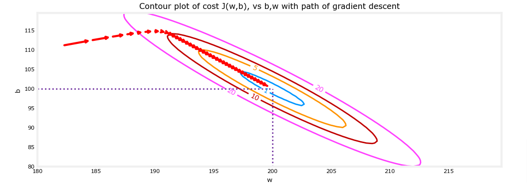
Learning Rate
As we discussed above if we start with a large learning rate there is a possibility that we may never converge and possibly diverge.
# initialize parameters
w_init = 0
b_init = 0
# set alpha to a large value
iterations = 10
tmp_alpha = 8.0e-1
# run gradient descent
w_final, b_final, J_hist, p_hist = gradient_descent(x_train ,y_train, w_init, b_init, tmp_alpha,
                                                    iterations, compute_cost, compute_gradient)
Above, w and b are bouncing back and forth between positive and negative with the absolute value increasing with each iteration. Further, each iteration ∂J(w,b)∂w changes sign and cost is increasing rather than decreasing. This is a clear sign that the learning rate is too large and the solution is diverging. Let’s visualize this with a plot.
plt_divergence(p_hist, J_hist,x_train, y_train)
plt.show()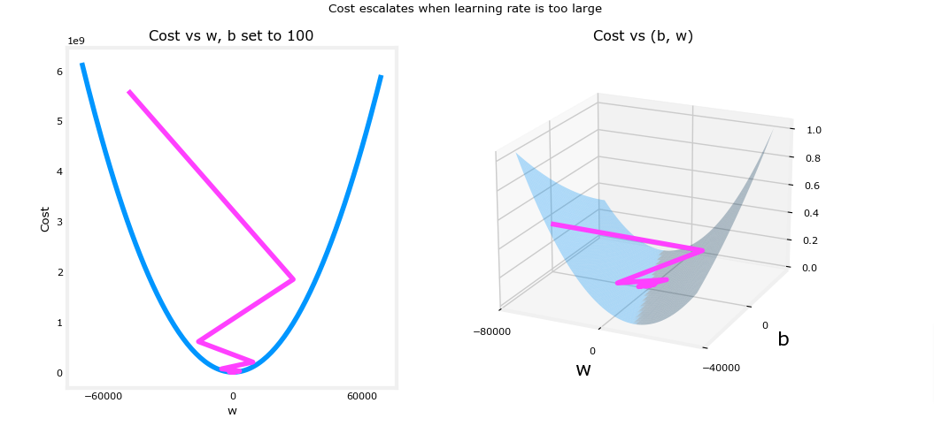
Above, the left graph shows w’s progression over the first few steps of gradient descent. w oscillates from positive to negative and cost grows rapidly. Gradient Descent is operating on both w and b simultaneously, so one needs the 3-D plot on the right for the complete picture.