NN in Numpy - Coffee Roasting

We will build a small NN using Numpy. It will be implemented again in TF in the next page.

Setup

import numpy as np
import matplotlib.pyplot as plt
plt.style.use('./deeplearning.mplstyle')
import tensorflow as tf
from lab_utils_common import dlc, sigmoid
from lab_coffee_utils import load_coffee_data, plt_roast, plt_prob, plt_layer, plt_network, plt_output_unit
import logging
logging.getLogger("tensorflow").setLevel(logging.ERROR)
tf.autograph.set_verbosity(0)

.

Dataset

def load_coffee_data():
    """ Creates a coffee roasting data set.
        roasting duration: 12-15 minutes is best
        temperature range: 175-260C is best
    """
    rng = np.random.default_rng(2)
    X = rng.random(400).reshape(-1,2)
    X[:,1] = X[:,1] * 4 + 11.5          # 12-15 min is best
    X[:,0] = X[:,0] * (285-150) + 150  # 350-500 F (175-260 C) is best
    Y = np.zeros(len(X))
    
    i=0
    for t,d in X:
        y = -3/(260-175)*t + 21
        if (t > 175 and t < 260 and d > 12 and d < 15 and d<=y ):
            Y[i] = 1
        else:
            Y[i] = 0
        i += 1

    return (X, Y.reshape(-1,1))

X,Y = load_coffee_data();
print(X.shape, Y.shape)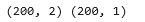

View

plt_roast(X,Y)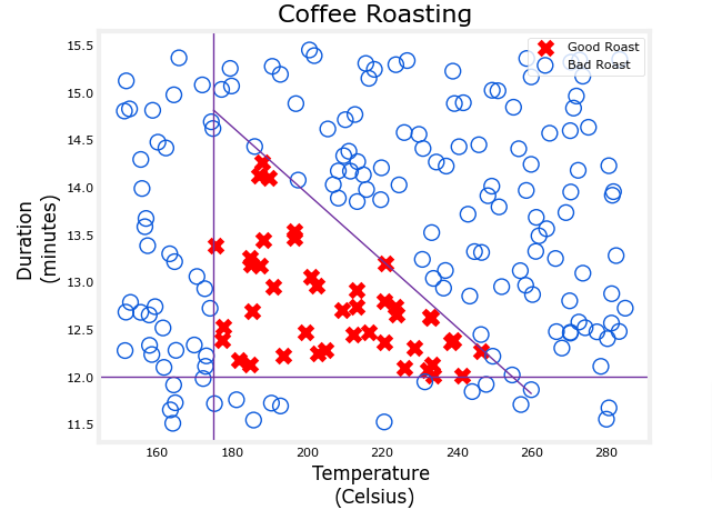

Normalize Data

print(f"Temperature Max, Min pre normalization: {np.max(X[:,0]):0.2f}, {np.min(X[:,0]):0.2f}")
print(f"Duration    Max, Min pre normalization: {np.max(X[:,1]):0.2f}, {np.min(X[:,1]):0.2f}")
norm_l = tf.keras.layers.Normalization(axis=-1)
norm_l.adapt(X)  # learns mean, variance
Xn = norm_l(X)
print(f"Temperature Max, Min post normalization: {np.max(Xn[:,0]):0.2f}, {np.min(Xn[:,0]):0.2f}")
print(f"Duration    Max, Min post normalization: {np.max(Xn[:,1]):0.2f}, {np.min(Xn[:,1]):0.2f}")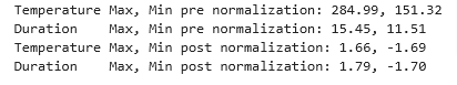

Build Model

---

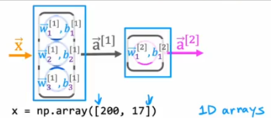
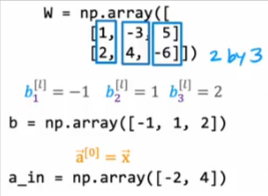
From previous pages we know the following:

• Here are the formulas for a1

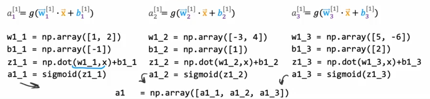
• We have to compute a2 next

Build Layers

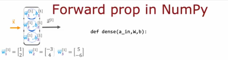
So we’ll take the w and b values and stack them into arrays and use them in the dense function and you’ll see the code and image below

A layer simply contains multiple neurons/units we will define the function below:

• One can utilize a for loop to visit each unit (j) in the layer and perform the dot product of the weights for that unit (W[:,j]) and sum the bias for the unit (b[j]) to form z.
• An activation function g(z) can then be applied to that result. Let’s try that below to build a “dense layer” subroutine.

def my_dense(a_in, W, b, g):
    """
    Computes dense layer
    Args:
      a_in (ndarray (n, )) : Data, 1 example 
      W    (ndarray (n,j)) : Weight matrix, n features per unit, j units
      b    (ndarray (j, )) : bias vector, j units  
      g    activation function (e.g. sigmoid, relu..)
    Returns
      a_out (ndarray (j,))  : j units|
    """
    units = W.shape[1]
    a_out = np.zeros(units)
    for j in range(units):               
        w = W[:,j]                                    
        z = np.dot(w, a_in) + b[j]         
        a_out[j] = g(z)               
    return(a_out)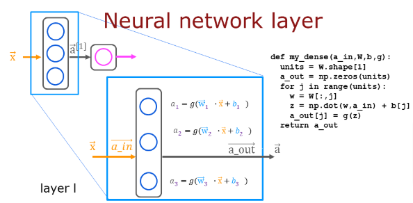

A quick test

# Quick Check
x_tst = 0.1*np.arange(1,3,1).reshape(2,)  # (1 examples, 2 features)
W_tst = 0.1*np.arange(1,7,1).reshape(2,3) # (2 input features, 3 output features)
b_tst = 0.1*np.arange(1,4,1).reshape(3,)  # (3 features)
A_tst = my_dense(x_tst, W_tst, b_tst, sigmoid)
print(A_tst)

The following cell builds a two-layer neural network utilizing the my_dense subroutine above.

• Here is how we can string together layers sequentially to create the model

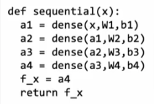
def my_sequential(x, W1, b1, W2, b2):
    a1 = my_dense(x,  W1, b1, sigmoid)
    a2 = my_dense(a1, W2, b2, sigmoid)
    return(a2)

Get trained weights and biases from the TF project for same idea

W1_tmp = np.array( [[-8.93,  0.29, 12.9 ], [-0.1,  -7.32, 10.81]] )
b1_tmp = np.array( [-9.82, -9.28,  0.96] )
W2_tmp = np.array( [[-31.18], [-27.59], [-32.56]] )
b2_tmp = np.array( [15.41] )

Predictions

---

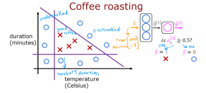
Once you have a trained model, you can then use it to make predictions. Recall that the output of our model is a probability. In this case, the probability of a good roast. To make a decision, one must apply the probability to a threshold. In this case, we will use 0.5

Let’s start by writing a routine similar to Tensorflow’s model.predict(). This will take a matrix X with all m examples in the rows and make a prediction by running the model.

def my_predict(X, W1, b1, W2, b2):
    m = X.shape[0]
    p = np.zeros((m,1))
    for i in range(m):
        p[i,0] = my_sequential(X[i], W1, b1, W2, b2)
    return(p)

Let’s try it on two examples

X_tst = np.array([
    [200,13.9],  # postive example
    [200,17]])   # negative example
X_tstn = norm_l(X_tst)  # remember to normalize
predictions = my_predict(X_tstn, W1_tmp, b1_tmp, W2_tmp, b2_tmp)

Convert the probability to a decision, apply a threshold

yhat = np.zeros_like(predictions)
for i in range(len(predictions)):
    if predictions[i] >= 0.5:
        yhat[i] = 1
    else:
        yhat[i] = 0
print(f"decisions = \n{yhat}")

or

yhat = (predictions >= 0.5).astype(int)
print(f"decisions = \n{yhat}")

Plot

---

This graph shows the operation of the whole network and is identical to the Tensorflow result from the previous lab. The left graph is the raw output of the final layer represented by the blue shading. This is overlaid on the training data represented by the X’s and O’s.
The right graph is the output of the network after a decision threshold. The X’s and O’s here correspond to decisions made by the network.

netf= lambda x : my_predict(norm_l(x),W1_tmp, b1_tmp, W2_tmp, b2_tmp)
plt_network(X,Y,netf)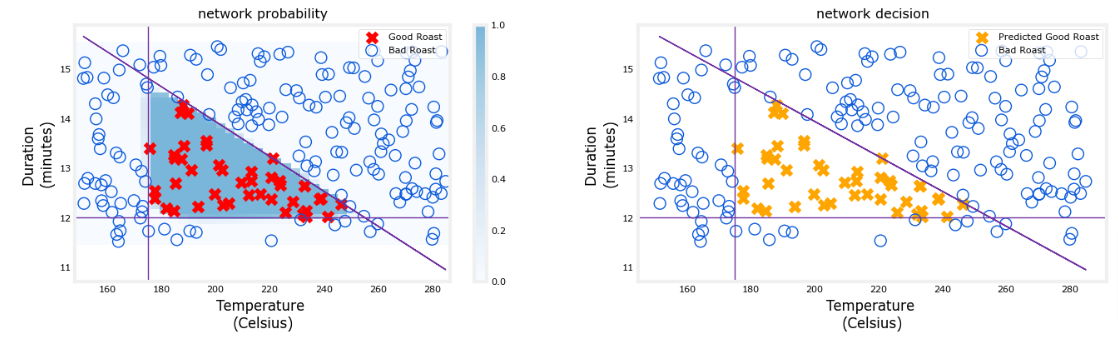

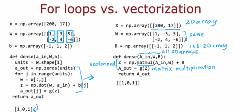
Vectorization

---

Vectorization allows us to speed NN models and allows us to process them in CPUs at times faster than before. Here we see the difference using matrices instead of arrays.