import numpy as np    # it is an unofficial standard to use np for numpy
import timeMultiple LR
My thanks and credit to Stanford University & Andrew Ng for their contributions.
We will extend the data structures we previously used to develop the functions for single feature linear regression.
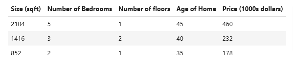
So let’s improve on our dataset to include four features, size, bedrooms, floors, and age so we can include these features when we are trying to predict the value of a house, hoping it will give us a more accurate prediction.
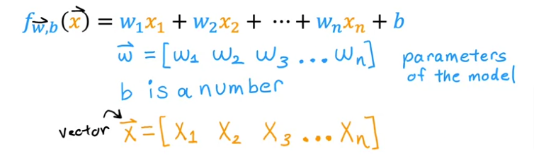
Notations
New Notations
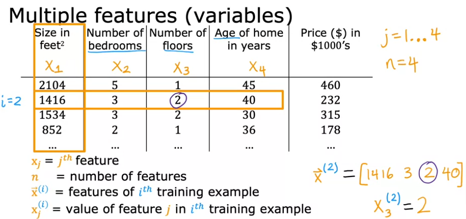
- The first thing we need to do is edit our notation so we can include an infinite number of features to x1, x2, x3, x4 and so on…. with xj = jth feature regardless how many (j) features we have or for simplicity let’s call
- n = number of features = 4
- A vector -> \(\vec{x}^{(i)}\) = features of ith training example or the features in the ith row. Sometimes we call it a row vector
- To extract one value of one of the features, we have to specify its row and column and we can do that by using the vector notation for the column j in the row i as: x(i)j
- Or to remember it better: xcolumn(row)
Recap
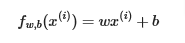
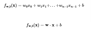
The linear model with one variable is given by
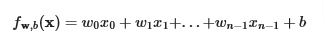
The linear model with n variables is given by. The reason we end with n-1 is because vector and matrix notations in Numpy start with 0 and therefore the length of n len(n) is n-1
Here is one way of looking at it:
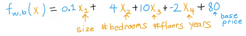
- 0.1 is the size multiplier, so we are saying that if a house increases by 1000 ft2 it will increase by 0.1X1000=$100 so we can estimate the importance to the overall value of the price of the house by adjusting the factor for that specific feature.
- So for each additional bedroom the price increases by 4000….
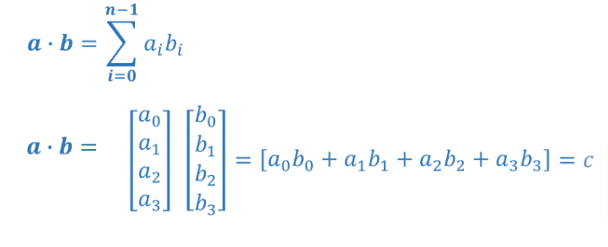
Vectorization
Will suffice to say for now that it is much more efficient to use vectors to make the calculations, we’ll get into why later. We can use GPUs to process vector operations which speed up the process. For now let’s cover what a vector is.
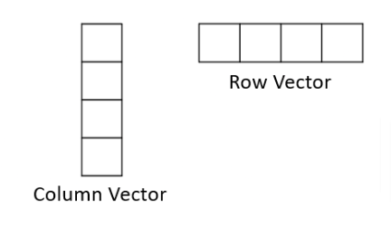
If you remember from Numpy that a vector is a 1D array. Depending on the orientation of the data, it could be a row vector or a column vector
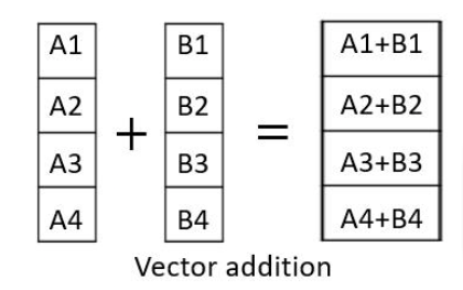
You can add, multiply or subtract vectors (column or rows) by going across what’s important is that the two/n vectors we are performing the operation on should be of equal length (same size)
- So going back to our dataset and formula for linear regression we can represent everything with vectors like this
- Now we can rewrite our regression model as

Code
Refer to Numpy page for more information
.
Numpy Array
# NumPy routines which allocate memory and fill with user specified values
a = np.array([5,4,3,2]);  print(f"np.array([5,4,3,2]):  a = {a},     a shape = {a.shape}, a data type = {a.dtype}, a type = {type(a)}")
np.array([5,4,3,2]): a = [5 4 3 2], a shape = (4,), a data type = int64, a type = <class 'numpy.ndarray'>Dot Product
.
Slow function
def my_dot(a, b):
    """
   Compute the dot product of two vectors

    Args:
      a (ndarray (n,)):  input vector
      b (ndarray (n,)):  input vector with same dimension as a

    Returns:
      x (scalar):
    """
    x=0
    for i in range(a.shape[0]):
        x = x + a[i] * b[i]
    return x
# test 1-D
a = np.array([1, 2, 3, 4])
b = np.array([-1, 4, 3, 2])
print(f"my_dot(a, b) = {my_dot(a, b)}")my_dot(a, b) = 24Use np.dot
# test 1-D
a = np.array([1, 2, 3, 4])
b = np.array([-1, 4, 3, 2])
c = np.dot(a, b)
print(f"NumPy 1-D np.dot(a, b) = {c}, np.dot(a, b).shape = {c.shape} ")
c = np.dot(b, a)
print(f"NumPy 1-D np.dot(b, a) = {c}, np.dot(a, b).shape = {c.shape} ")
NumPy 1-D np.dot(a, b) = 24, np.dot(a, b).shape = ()
NumPy 1-D np.dot(b, a) = 24, np.dot(a, b).shape = () Our data will be stored in an array or extracted from a dataframe as a vector. Note that since w is a 1-dimensional vector we can only multiply it with one parameter so we used x[1] which is a one dimensional vector
# show common Course 1 example
X = np.array([[1],[2],[3],[4]])
w = np.array([2])
c = np.dot(X[1], w)

print(f"X[1] has shape {X[1].shape}")
print(f"w has shape {w.shape}")
print(f"c has shape {c.shape}")
X[1] has shape (1,)
w has shape (1,)
c has shape ()Predict Target
So let’s use the data from above
import copy, math
import numpy as np
import matplotlib.pyplot as plt
plt.style.use('./deeplearning.mplstyle')
np.set_printoptions(precision=2)  # reduced display precision on numpy arrays
You see below the features are xn(i) where n is the number of features (4), and (i) is the the row in which the value is extracted from. (i) is a value of m the total number of rows/training samples. Remember (m,n) are the number of rows and columns respectively
X_train = np.array([[2104, 5, 1, 45], [1416, 3, 2, 40], [852, 2, 1, 35]])
y_train = np.array([460, 232, 178])
Let’s look at the data
- remember m is the number or rows, n number of columns so x (features) should be a (3,4) matrix
- the target column (y) is just an array of 3 elements so it would be (3,) 3 rows and one column, but since its an array the 1 is omitted (3,)
# data is stored in numpy array/matrix
print(f"X Shape: {X_train.shape}, X Type:{type(X_train)})")
print(X_train)
print(f"y Shape: {y_train.shape}, y Type:{type(y_train)})")
print(y_train)
X Shape: (3, 4), X Type:<class 'numpy.ndarray'>)
[[2104 5 1 45]
[1416 3 2 40]
[ 852 2 1 35]]
y Shape: (3,), y Type:<class 'numpy.ndarray'>)
[460 232 178]- Unlike the single variable LR in this case w is a vector and has to be the same size as all the features for x or the number of columns containing all the features, in this case n so it would be (4,)
- Remember the data set has 5 columns in total but one of them is the target value, y and therefore it is not counted when counting the number of x (features)
- So let’s guess at the initial values for w & b
b_init = 785.1811367994083
w_init = np.array([ 0.39133535, 18.75376741, -53.36032453, -26.42131618])
print(f"w_init shape: {w_init.shape}, b_init type: {type(b_init)}")
w_init shape: (4,), b_init type: <class 'float'>Predict without dot
Once again remember the formulas
Let’s extract one row of x’s and predict the value of y(price of house) and see how close we get to the actual value
Since we are only predicting the value based on one row (4 features) we can use simple math to process it instead of dot()
# Not dot prediction function
def predict_single_loop(x, w, b):
    """
    single predict using linear regression

    Args:
      x (ndarray): Shape (n,) example with multiple features
      w (ndarray): Shape (n,) model parameters
      b (scalar):  model parameter

    Returns:
      p (scalar):  prediction
    """
    n = x.shape[0]
    p = 0
    for i in range(n):
        p_i = x[i] * w[i]
        p = p + p_i
    p = p + b
    return p
# extract one row from our training data
x_vec = X_train[0,:]
print(f"x_vec shape {x_vec.shape}, x_vec value: {x_vec}")x_vec shape (4,), x_vec value: [2104 5 1 45]# make the prediction using the formula shown above in the image
f_wb = predict_single_loop(x_vec, w_init, b_init)
print(f"f_wb shape {f_wb.shape}, prediction: {f_wb}")f_wb shape (), prediction: 459.9999976194083Predict with dot
Of course the answer would be the same as before
# dot prediction function
def predict(x, w, b):
    """
    single predict using linear regression
    Args:
      x (ndarray): Shape (n,) example with multiple features
      w (ndarray): Shape (n,) model parameters
      b (scalar):             model parameter

    Returns:
      p (scalar):  prediction
    """
    p = np.dot(x, w) + b
    return p
# get a row from our training data
x_vec = X_train[0,:]
print(f"x_vec shape {x_vec.shape}, x_vec value: {x_vec}")
# make a prediction
f_wb = predict(x_vec,w_init, b_init)
print(f"f_wb shape {f_wb.shape}, prediction: {f_wb}")x_vec shape (4,), x_vec value: [2104 5 1 45]
f_wb shape (), prediction: 459.9999976194083