NN for Content-Filtering Movies

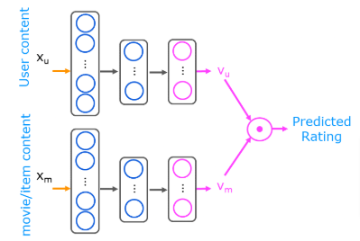
We will construct two NN one for movie content and one for user content. We will then combine the two using dot product to predict a value and present recommendations based on the predictions.

Movie Dataset

---

The data set is derived from the MovieLens ml-latest-small dataset.

[F. Maxwell Harper and Joseph A. Konstan. 2015. The MovieLens Datasets: History and Context. ACM Transactions on Interactive Intelligent Systems (TiiS) 5, 4: 19:1–19:19. https://doi.org/10.1145/2827872]

The original dataset has roughly 9000 movies rated by 600 users with ratings on a scale of 0.5 to 5 in 0.5 step increments. The dataset has been reduced in size to focus on movies from the years since 2000 and popular genres. The reduced dataset has 𝑛𝑢=397nu=397 users, 𝑛𝑚=847nm=847 movies and 25521 ratings. For each movie, the dataset provides a movie title, release date, and one or more genres. For example “Toy Story 3” was released in 2010 and has several genres: “Adventure|Animation|Children|Comedy|Fantasy”. This dataset contains little information about users other than their ratings. This dataset is used to create training vectors for the neural networks described below. Let’s learn a bit more about this data set. The table below shows the top 10 movies ranked by the number of ratings. These movies also happen to have high average ratings.

import numpy as np
import numpy.ma as ma
import pandas as pd
import tensorflow as tf
from tensorflow import keras
from sklearn.preprocessing import StandardScaler, MinMaxScaler
from sklearn.model_selection import train_test_split
import tabulate
from recsysNN_utils import *
pd.set_option("display.precision", 1)

top10_df = pd.read_csv("./data/content_top10_df.csv")
bygenre_df = pd.read_csv("./data/content_bygenre_df.csv")
top10_df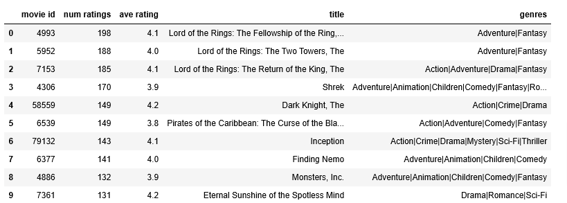

Here is information sorted by genre.

• The number of ratings vary substantially.
• A movie might have several genres so the sum of the ratings might be larger

bygenre_df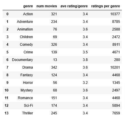

The original features are the year the movie was released and the movie’s genre’s presented as a one-hot vector. There are 14 genres. The engineered feature is an average rating derived from the user ratings.

The user content is composed of engineered features. A per genre average rating is computed per user. Additionally, a user id, rating count and rating average are available but not included in the training or prediction content. They are carried with the data set because they are useful in interpreting data.

The training set consists of all the ratings made by the users in the data set. Some ratings are repeated to boost the number of training examples of underrepresented genre’s. The training set is split into two arrays with the same number of entries, a user array and a movie/item array.

Below, let’s load and display some of the data.

# Load Data, set configuration variables
item_train, user_train, y_train, item_features, user_features, item_vecs, movie_dict, user_to_genre = load_data()

num_user_features = user_train.shape[1] - 3  # remove userid, rating count and ave rating during training
num_item_features = item_train.shape[1] - 1  # remove movie id at train time
uvs = 3  # user genre vector start
ivs = 3  # item genre vector start
u_s = 3  # start of columns to use in training, user
i_s = 1  # start of columns to use in training, items
print(f"Number of training vectors: {len(item_train)}")

Number of training vectors: 50884

Preview Training Array

Lets look at some of the user features

pprint_train(user_train, user_features, uvs,  u_s, maxcount=5)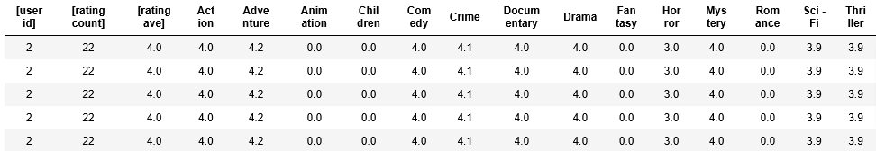

Some of the user and item/movie features are not used in training. In the table above, the features in brackets “[]” such as the “user id”, “rating count” and “rating ave” are not included when the model is trained and used.

Above you can see the per genre rating average for user 2. Zero entries are genre’s which the user had not rated. The user vector is the same for all the movies rated by a user.

Let’s look at the first few entries of the movie/item array.

pprint_train(item_train, item_features, ivs, i_s, maxcount=5, user=False)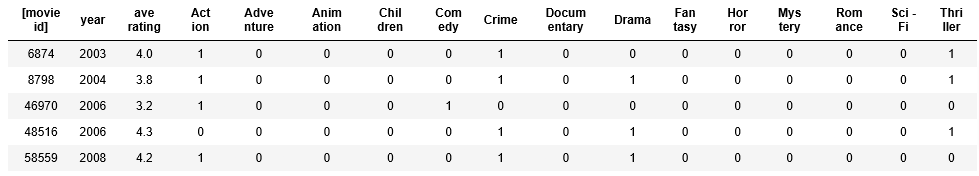

Above, the movie array contains the year the film was released, the average rating and an indicator for each potential genre. The indicator is one for each genre that applies to the movie. The movie id is not used in training but is useful when interpreting the data.

print(f"y_train[:5]: {y_train[:5]}")

y_train[:5]: [4.  3.5 4.  4.  4.5]

The target, y, is the movie rating given by the user.

Above, we can see that movie 6874 is an Action/Crime/Thriller movie released in 2003. User 2 rates action movies as 3.9 on average. MovieLens users gave the movie an average rating of 4. ‘y’ is 4 indicating user 2 rated movie 6874 as a 4 as well. A single training example consists of a row from both the user and item arrays and a rating from y_train.

Scale Training Data

---

 Below, the inverse_transform is also shown to produce the original inputs. We’ll scale the target ratings using a Min Max Scaler which scales the target to be between -1 and 1. scikit learn MinMaxScaler

# scale training data
item_train_unscaled = item_train
user_train_unscaled = user_train
y_train_unscaled    = y_train

scalerItem = StandardScaler()
scalerItem.fit(item_train)
item_train = scalerItem.transform(item_train)

scalerUser = StandardScaler()
scalerUser.fit(user_train)
user_train = scalerUser.transform(user_train)

scalerTarget = MinMaxScaler((-1, 1))
scalerTarget.fit(y_train.reshape(-1, 1))
y_train = scalerTarget.transform(y_train.reshape(-1, 1))
#ynorm_test = scalerTarget.transform(y_test.reshape(-1, 1))

print(np.allclose(item_train_unscaled, scalerItem.inverse_transform(item_train)))
print(np.allclose(user_train_unscaled, scalerUser.inverse_transform(user_train)))

True
True

Split Data

---

To allow us to evaluate the results, we will split the data into training and test sets. Here we will use sklean train_test_split to split and shuffle the data. Note that setting the initial random state to the same value ensures item, user, and y are shuffled identically

item_train, item_test = train_test_split(item_train, train_size=0.80, shuffle=True, random_state=1)
user_train, user_test = train_test_split(user_train, train_size=0.80, shuffle=True, random_state=1)
y_train, y_test       = train_test_split(y_train,    train_size=0.80, shuffle=True, random_state=1)
print(f"movie/item training data shape: {item_train.shape}")
print(f"movie/item test data shape: {item_test.shape}")

movie/item training data shape: (40707, 17)
movie/item test data shape: (10177, 17)

The scaled, shuffled data now has a mean of 0 as expected.

pprint_train(user_train, user_features, uvs, u_s, maxcount=5)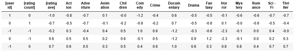

Neural Network

---

Construct a neural network as described in the figure above. It will have two networks that are combined by a dot product. You will construct the two networks. In this example, they will be identical. Note that these networks do not need to be the same. If the user content was substantially larger than the movie content, you might elect to increase the complexity of the user network relative to the movie network. In this case, the content is similar, so the networks are the same.

Use a Keras sequential model

• The first layer is a dense layer with 256 units and a relu activation.
• The second layer is a dense layer with 128 units and a relu activation.
• The third layer is a dense layer with num_outputs units and a linear or no activation.

num_outputs = 32
tf.random.set_seed(1)
user_NN = tf.keras.models.Sequential([
  tf.keras.layers.Dense(256, activation='relu'),
  tf.keras.layers.Dense(128, activation='relu'),
  tf.keras.layers.Dense(num_outputs)
])

item_NN = tf.keras.models.Sequential([
  tf.keras.layers.Dense(256, activation='relu'),
  tf.keras.layers.Dense(128, activation='relu'),
  tf.keras.layers.Dense(num_outputs)  
])

# create the user input and point to the base network
input_user = tf.keras.layers.Input(shape=(num_user_features))
vu = user_NN(input_user)
vu = tf.linalg.l2_normalize(vu, axis=1)

# create the item input and point to the base network
input_item = tf.keras.layers.Input(shape=(num_item_features))
vm = item_NN(input_item)
vm = tf.linalg.l2_normalize(vm, axis=1)

# compute the dot product of the two vectors vu and vm
output = tf.keras.layers.Dot(axes=1)([vu, vm])

# specify the inputs and output of the model
model = tf.keras.Model([input_user, input_item], output)

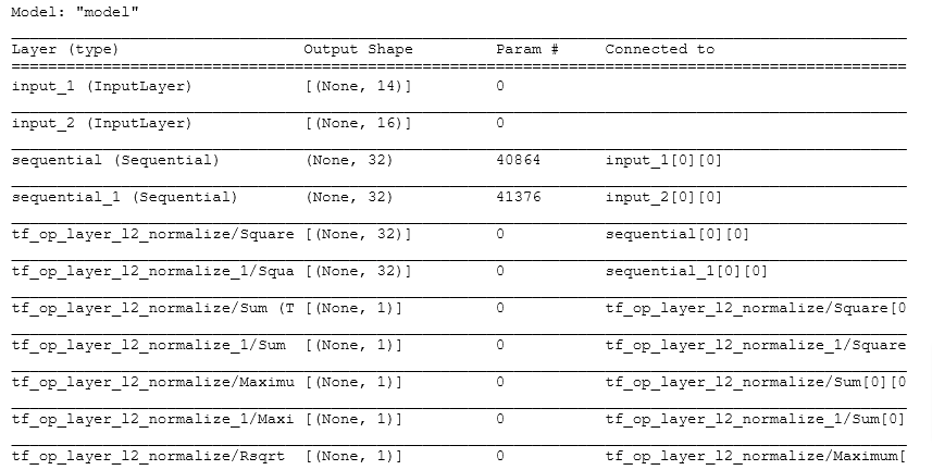
model.summary()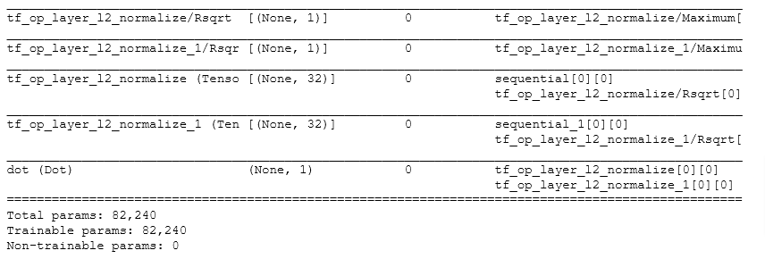

Mean Square Error & Adam

tf.random.set_seed(1)
cost_fn = tf.keras.losses.MeanSquaredError()
opt = keras.optimizers.Adam(learning_rate=0.01)
model.compile(optimizer=opt,
              loss=cost_fn)

Train Model

# Train model
tf.random.set_seed(1)
model.fit([user_train[:, u_s:], item_train[:, i_s:]], y_train, epochs=30)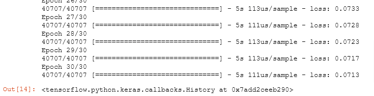

Evaluate Model

# Evaluate on test data
model.evaluate([user_test[:, u_s:], item_test[:, i_s:]], y_test)

It is comparable to the training loss indicating the model has not substantially overfit the training data.

Predictions

---

New User

First, we’ll create a new user and have the model suggest movies for that user. After you have tried this on the example user content, feel free to change the user content to match your own preferences and see what the model suggests. Note that ratings are between 0.5 and 5.0, inclusive, in half-step increments

new_user_id = 5000
new_rating_ave = 0.0
new_action = 0.0
new_adventure = 5.0
new_animation = 0.0
new_childrens = 0.0
new_comedy = 0.0
new_crime = 0.0
new_documentary = 0.0
new_drama = 0.0
new_fantasy = 5.0
new_horror = 0.0
new_mystery = 0.0
new_romance = 0.0
new_scifi = 0.0
new_thriller = 0.0
new_rating_count = 3

user_vec = np.array([[new_user_id, new_rating_count, new_rating_ave,
                      new_action, new_adventure, new_animation, new_childrens,
                      new_comedy, new_crime, new_documentary,
                      new_drama, new_fantasy, new_horror, new_mystery,
                      new_romance, new_scifi, new_thriller]])

The new user enjoys movies from the adventure, fantasy genres. Let’s find the top-rated movies for the new user.
Below, we’ll use a set of movie/item vectors, item_vecs that have a vector for each movie in the training/test set. This is matched with the new user vector above and the scaled vectors are used to predict ratings for all the movies.

# generate and replicate the user vector to match the number movies in the data set.
user_vecs = gen_user_vecs(user_vec,len(item_vecs))

# scale our user and item vectors
suser_vecs = scalerUser.transform(user_vecs)
sitem_vecs = scalerItem.transform(item_vecs)

# make a prediction
y_p = model.predict([suser_vecs[:, u_s:], sitem_vecs[:, i_s:]])

# unscale y prediction 
y_pu = scalerTarget.inverse_transform(y_p)

# sort the results, highest prediction first
sorted_index = np.argsort(-y_pu,axis=0).reshape(-1).tolist()  #negate to get largest rating first
sorted_ypu   = y_pu[sorted_index]
sorted_items = item_vecs[sorted_index]  #using unscaled vectors for display

print_pred_movies(sorted_ypu, sorted_items, movie_dict, maxcount = 10)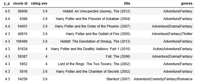

Existing User

Let’s look at the predictions for “user 2”, one of the users in the data set. We can compare the predicted ratings with the model’s ratings

uid = 2 
# form a set of user vectors. This is the same vector, transformed and repeated.
user_vecs, y_vecs = get_user_vecs(uid, user_train_unscaled, item_vecs, user_to_genre)

# scale our user and item vectors
suser_vecs = scalerUser.transform(user_vecs)
sitem_vecs = scalerItem.transform(item_vecs)

# make a prediction
y_p = model.predict([suser_vecs[:, u_s:], sitem_vecs[:, i_s:]])

# unscale y prediction 
y_pu = scalerTarget.inverse_transform(y_p)

# sort the results, highest prediction first
sorted_index = np.argsort(-y_pu,axis=0).reshape(-1).tolist()  #negate to get largest rating first
sorted_ypu   = y_pu[sorted_index]
sorted_items = item_vecs[sorted_index]  #using unscaled vectors for display
sorted_user  = user_vecs[sorted_index]
sorted_y     = y_vecs[sorted_index]

#print sorted predictions for movies rated by the user
print_existing_user(sorted_ypu, sorted_y.reshape(-1,1), sorted_user, sorted_items, ivs, uvs, movie_dict, maxcount = 50)

The model prediction is generally within 1 of the actual rating though it is not a very accurate predictor of how a user rates specific movies. This is especially true if the user rating is significantly different than the user’s genre average. You can vary the user id above to try different users. Not all user id’s were used in the training set.

Find Similar Items

---

The neural network above produces two feature vectors, a user feature vector 𝑣𝑢vu, and a movie feature vector, 𝑣𝑚vm. These are 32 entry vectors whose values are difficult to interpret. However, similar items will have similar vectors. This information can be used to make recommendations. For example, if a user has rated “Toy Story 3” highly, one could recommend similar movies by selecting movies with similar movie feature vectors.

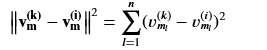
A similarity measure is the squared distance between the two vectors 𝐯(𝐤)𝐦vm(k) and 𝐯(𝐢)𝐦vm(i)

Compute Square Distance

def sq_dist(a,b):
    """
    Returns the squared distance between two vectors
    Args:
      a (ndarray (n,)): vector with n features
      b (ndarray (n,)): vector with n features
    Returns:
      d (float) : distance
    """
    d = np.sum((a - b)**2)    
    return d

a1 = np.array([1.0, 2.0, 3.0]); b1 = np.array([1.0, 2.0, 3.0])
a2 = np.array([1.1, 2.1, 3.1]); b2 = np.array([1.0, 2.0, 3.0])
a3 = np.array([0, 1, 0]);       b3 = np.array([1, 0, 0])
print(f"squared distance between a1 and b1: {sq_dist(a1, b1):0.3f}")
print(f"squared distance between a2 and b2: {sq_dist(a2, b2):0.3f}")
print(f"squared distance between a3 and b3: {sq_dist(a3, b3):0.3f}")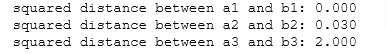

Calculate Distance Matrix

A matrix of distances between movies can be computed once when the model is trained and then reused for new recommendations without retraining. The first step, once a model is trained, is to obtain the movie feature vector, 𝑣𝑚vm, for each of the movies. To do this, we will use the trained item_NN and build a small model to allow us to run the movie vectors through it to generate 𝑣𝑚vm.

input_item_m = tf.keras.layers.Input(shape=(num_item_features))    # input layer
vm_m = item_NN(input_item_m)                                       # use the trained item_NN
vm_m = tf.linalg.l2_normalize(vm_m, axis=1)                        # incorporate normalization as was done in the original model
model_m = tf.keras.Model(input_item_m, vm_m)                                
model_m.summary()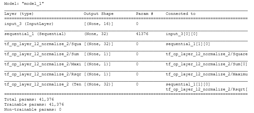

Movie Feature Vector

Once you have a movie model, you can create a set of movie feature vectors by using the model to predict using a set of item/movie vectors as input. item_vecs is a set of all of the movie vectors. It must be scaled to use with the trained model. The result of the prediction is a 32 entry feature vector for each movie.

scaled_item_vecs = scalerItem.transform(item_vecs)
vms = model_m.predict(scaled_item_vecs[:,i_s:])
print(f"size of all predicted movie feature vectors: {vms.shape}")

size of all predicted movie feature vectors: (847, 32)

Squared Distance Matrix

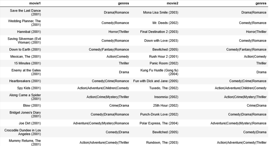
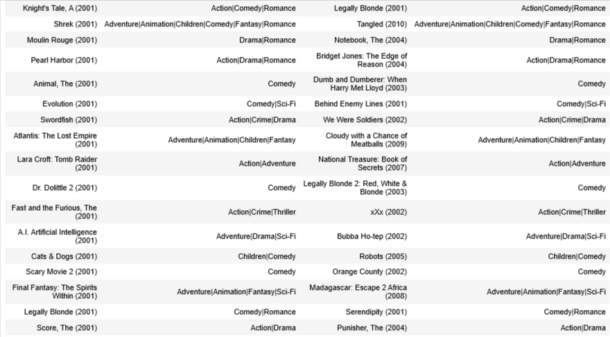
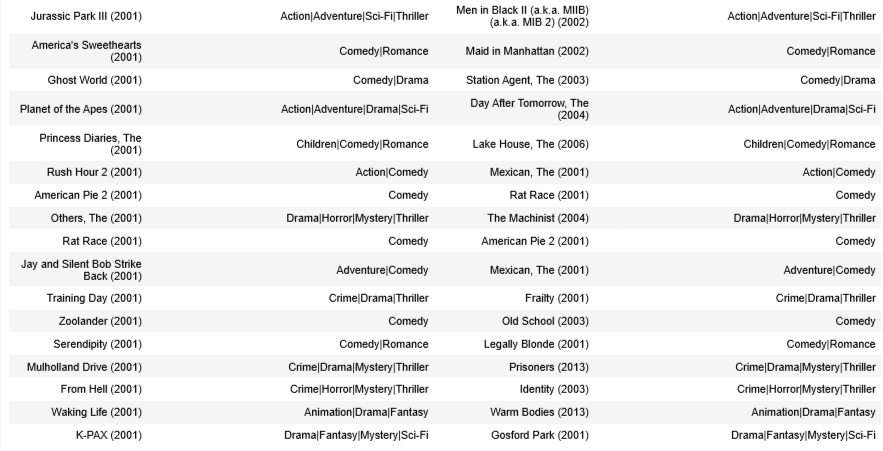
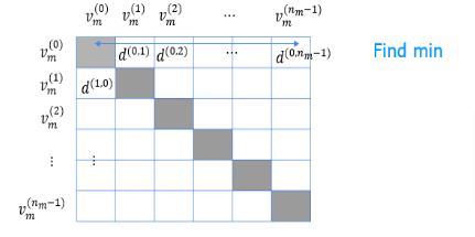
• Let’s compute a matrix of the squared distance between each movie feature vector and all other movie feature vectors
• We can then find the closest movie by finding the minimum along each row.
• We will make use of numpy masked arrays to avoid selecting the same movie. The masked values along the diagonal won’t be included in the computation.

count = 50  # number of movies to display
dim = len(vms)
dist = np.zeros((dim,dim))

for i in range(dim):
    for j in range(dim):
        dist[i,j] = sq_dist(vms[i, :], vms[j, :])
        
m_dist = ma.masked_array(dist, mask=np.identity(dist.shape[0]))  # mask the diagonal

disp = [["movie1", "genres", "movie2", "genres"]]
for i in range(count):
    min_idx = np.argmin(m_dist[i])
    movie1_id = int(item_vecs[i,0])
    movie2_id = int(item_vecs[min_idx,0])
    disp.append( [movie_dict[movie1_id]['title'], movie_dict[movie1_id]['genres'],
                  movie_dict[movie2_id]['title'], movie_dict[movie1_id]['genres']]
               )
table = tabulate.tabulate(disp, tablefmt='html', headers="firstrow")
table