Data

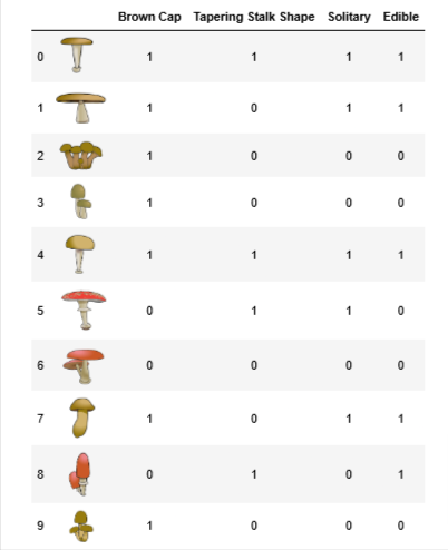
Edible vs Poisonous Mushrooms

Suppose you are starting a company that grows and sells wild mushrooms.

• Since not all mushrooms are edible, you’d like to be able to tell whether a given mushroom is edible or poisonous based on it’s physical attributes
• You have some existing data that you can use for this task.

Can you use the data to help you identify which mushrooms can be sold safely?

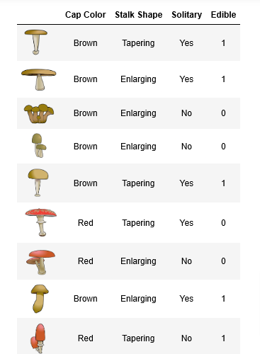
Data

• You have 10 examples of mushrooms. For each example, you have

  • Three features

    • Cap Color (Brown or Red),

    • Stalk Shape (Tapering (as in \/) or Enlarging (as in /\)), and

    • Solitary (Yes or No)

  • Label

    • Edible (1 indicating yes or 0 indicating poisonous)

One Hot Encoded

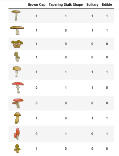
Therefore,

• X_train contains three features for each example

  • Brown Color (A value of 1 indicates “Brown” cap color and 0 indicates “Red” cap color)

  • Tapering Shape (A value of 1 indicates “Tapering Stalk Shape” and 0 indicates “Enlarging” stalk shape)

  • Solitary (A value of 1 indicates “Yes” and 0 indicates “No”)

• y_train is whether the mushroom is edible

  • y = 1 indicates edible

  • y = 0 indicates poisonous

Setup

import numpy as np
import matplotlib.pyplot as plt
from public_tests import *
from utils import *

%matplotlib inline

X_train = np.array([[1,1,1],[1,0,1],[1,0,0],[1,0,0],[1,1,1],[0,1,1],[0,0,0],[1,0,1],[0,1,0],[1,0,0]])
y_train = np.array([1,1,0,0,1,0,0,1,1,0])

print("First few elements of X_train:\n", X_train[:5])
print("Type of X_train:",type(X_train))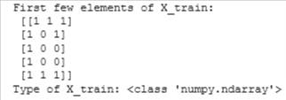

print("First few elements of y_train:", y_train[:5])
print("Type of y_train:",type(y_train))

print ('The shape of X_train is:', X_train.shape)
print ('The shape of y_train is: ', y_train.shape)
print ('Number of training examples (m):', len(X_train))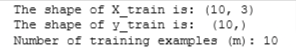

Steps to Build DT

Recall that the steps for building a decision tree are as follows:

• Start with all examples at the root node
• Calculate information gain for splitting on all possible features, and pick the one with the highest information gain
• Split dataset according to the selected feature, and create left and right branches of the tree
• Keep repeating splitting process until stopping criteria is met

Now we will implement the following functions, which will let you split a node into left and right branches using the feature with the highest information gain

• Calculate the entropy at a node
• Split the dataset at a node into left and right branches based on a given feature
• Calculate the information gain from splitting on a given feature
• Choose the feature that maximizes information gain
• We’ll then use the helper functions you’ve implemented to build a decision tree by repeating the splitting process until the stopping criteria is met
  • For this lab, the stopping criteria we’ve chosen is setting a maximum depth of 2

Entropy

First, you’ll write a helper function called compute_entropy that computes the entropy (measure of impurity) at a node.

• The function takes in a numpy array (y) that indicates whether the examples in that node are edible (1) or poisonous(0)

Complete the compute_entropy() function below to:

• Compute 𝑝1p1, which is the fraction of examples that are edible (i.e. have value = 1 in y)
• The entropy is then calculated as

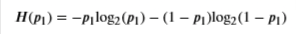
• The log is calculated with base 22
• For implementation purposes, 0log2(0)=00log2(0)=0. That is, if p_1 = 0 or p_1 = 1, set the entropy to 0
• Make sure to check that the data at a node is not empty (i.e. len(y) != 0). Return 0 if it is

To calculate p1

• You can get the subset of examples in y that have the value 1 as y[y == 1]
• You can use len(y) to get the number of examples in y

To calculate entropy

• np.log2 let’s you calculate the logarithm to base 2 for a numpy array
• If the value of p1 is 0 or 1, make sure to set the entropy to 0

def compute_entropy(y):
    """
    Computes the entropy for 
    
    Args:
       y (ndarray): Numpy array indicating whether each example at a node is
           edible (`1`) or poisonous (`0`)
       
    Returns:
        entropy (float): Entropy at that node
        
    """
    # You need to return the following variables correctly
    entropy = 0.
    
    if len(y) != 0:
     # Your code here to calculate the fraction of edible examples (i.e with value = 1 in y)
        p1 = len(y[y == 1]) / len(y)

     # For p1 = 0 and 1, set the entropy to 0 (to handle 0log0)
        if p1 != 0 and p1 != 1:
         # Your code here to calculate the entropy using the formula provided above
                entropy = -p1 * np.log2(p1) - (1- p1)*np.log2(1 - p1)
        else:
                entropy = 0        
    
    return entropy

# Compute entropy at the root node (i.e. with all examples)
# Since we have 5 edible and 5 non-edible mushrooms, the entropy should be 1"

print("Entropy at root node: ", compute_entropy(y_train)) 

# UNIT TESTS
compute_entropy_test(compute_entropy)

Split Dataset

Write a helper function called split_dataset that takes in the data at a node and a feature to split on and splits it into left and right branches. Later in the lab, you’ll implement code to calculate how good the split is.

• The function takes in the training data, the list of indices of data points at that node, along with the feature to split on.
• It splits the data and returns the subset of indices at the left and the right branch.
• For example, say we’re starting at the root node (so node_indices = [0,1,2,3,4,5,6,7,8,9]), and we chose to split on feature 0, which is whether or not the example has a brown cap.
• The output of the function is then, left_indices = [0,1,2,3,4,7,9] (data points with brown cap) and right_indices = [5,6,8] (data points without a brown cap)

• For each index in node_indices

  • If the value of X at that index for that feature is 1, add the index to left_indices

  • If the value of X at that index for that feature is 0, add the index to right_indices

def split_dataset(X, node_indices, feature):
    """
    Splits the data at the given node into
    left and right branches
    
    Args:
        X (ndarray):             Data matrix of shape(n_samples, n_features)
        node_indices (list):     List containing the active indices. I.e, the samples being considered at this step.
        feature (int):           Index of feature to split on
    
    Returns:
        left_indices (list):     Indices with feature value == 1
        right_indices (list):    Indices with feature value == 0
    """
    
    # You need to return the following variables correctly
    left_indices = []
    right_indices = []
    

    for i in node_indices:
        if X[i][feature] == 1:
            left_indices.append(i)
        else:
            right_indices.append(i)    

        
    return left_indices, right_indices

Let’s try splitting the dataset at the root node, which contains all examples at feature 0 (Brown Cap) as we’d discussed above. We’ve also provided a helper function to visualize the output of the split.

# Case 1

root_indices = [0, 1, 2, 3, 4, 5, 6, 7, 8, 9]

# Feel free to play around with these variables
# The dataset only has three features, so this value can be 0 (Brown Cap), 1 (Tapering Stalk Shape) or 2 (Solitary)
feature = 0

left_indices, right_indices = split_dataset(X_train, root_indices, feature)

print("CASE 1:")
print("Left indices: ", left_indices)
print("Right indices: ", right_indices)

# Visualize the split 
generate_split_viz(root_indices, left_indices, right_indices, feature)

print()

# Case 2

root_indices_subset = [0, 2, 4, 6, 8]
left_indices, right_indices = split_dataset(X_train, root_indices_subset, feature)

print("CASE 2:")
print("Left indices: ", left_indices)
print("Right indices: ", right_indices)

# Visualize the split 
generate_split_viz(root_indices_subset, left_indices, right_indices, feature)

# UNIT TESTS    
split_dataset_test(split_dataset)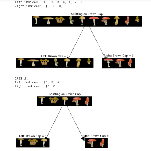

Information Gain

where

• 𝐻(𝑝node1)H(p1node) is entropy at the node
• 𝐻(𝑝left1)H(p1left) and 𝐻(𝑝right1)H(p1right) are the entropies at the left and the right branches resulting from the split
• 𝑤leftwleft and 𝑤rightwright are the proportion of examples at the left and right branch, respectively
• You can use the compute_entropy() function that you implemented above to calculate the entropy
• We’ve provided some starter code that uses the split_dataset() function you implemented above to split the dataset

def compute_information_gain(X, y, node_indices, feature):
    
    """
    Compute the information of splitting the node on a given feature
    
    Args:
        X (ndarray):            Data matrix of shape(n_samples, n_features)
        y (array like):         list or ndarray with n_samples containing the target variable
        node_indices (ndarray): List containing the active indices. I.e, the samples being considered in this step.
        feature (int):           Index of feature to split on
   
    Returns:
        cost (float):        Cost computed
    
    """    
    # Split dataset
    left_indices, right_indices = split_dataset(X, node_indices, feature)
    
    # Some useful variables
    X_node, y_node = X[node_indices], y[node_indices]
    X_left, y_left = X[left_indices], y[left_indices]
    X_right, y_right = X[right_indices], y[right_indices]
    
    # You need to return the following variables correctly
    information_gain = 0
    
    
    # Your code here to compute the entropy at the node using compute_entropy()
    node_entropy = compute_entropy(y_node)
    # Your code here to compute the entropy at the left branch
    left_entropy = compute_entropy(y_left)
    # Your code here to compute the entropy at the right branch
    right_entropy = compute_entropy(y_right)

    # Your code here to compute the proportion of examples at the left branch
    w_left = len(X_left) / len(X_node)

    # Your code here to compute the proportion of examples at the right branch
    w_right = len(X_right) / len(X_node)

    # Your code here to compute weighted entropy from the split using 
    # w_left, w_right, left_entropy and right_entropy
    weighted_entropy = w_left * left_entropy + w_right * right_entropy

    # Your code here to compute the information gain as the entropy at the node
    # minus the weighted entropy
    information_gain = node_entropy - weighted_entropy
    
    return information_gain

info_gain0 = compute_information_gain(X_train, y_train, root_indices, feature=0)
print("Information Gain from splitting the root on brown cap: ", info_gain0)

info_gain1 = compute_information_gain(X_train, y_train, root_indices, feature=1)
print("Information Gain from splitting the root on tapering stalk shape: ", info_gain1)

info_gain2 = compute_information_gain(X_train, y_train, root_indices, feature=2)
print("Information Gain from splitting the root on solitary: ", info_gain2)

Best Split

• The function takes in the training data, along with the indices of datapoint at that node
• The output of the function is the feature that gives the maximum information gain
  • You can use the compute_information_gain() function to iterate through the features and calculate the information for each feature If you get stuck, you can check out the hints presented after the cell below to help you with the implementation.

def get_best_split(X, y, node_indices):   
    """
    Returns the optimal feature and threshold value
    to split the node data 
    
    Args:
        X (ndarray):            Data matrix of shape(n_samples, n_features)
        y (array like):         list or ndarray with n_samples containing the target variable
        node_indices (ndarray): List containing the active indices. I.e, the samples being considered in this step.

    Returns:
        best_feature (int):     The index of the best feature to split
    """    
    
    # Some useful variables
    num_features = X.shape[1]
    
    # You need to return the following variables correctly
    best_feature = -1

    max_info_gain = 0

    # Iterate through all features
    for feature in range(num_features): 

       # Your code here to compute the information gain from splitting on this feature
       info_gain = compute_information_gain(X,y,node_indices,feature)

       # If the information gain is larger than the max seen so far
       if info_gain > max_info_gain:  
           # Your code here to set the max_info_gain and best_feature
           max_info_gain = info_gain
           best_feature =  feature  
   
   
    return best_feature

best_feature = get_best_split(X_train, y_train, root_indices)
print("Best feature to split on: %d" % best_feature)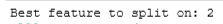

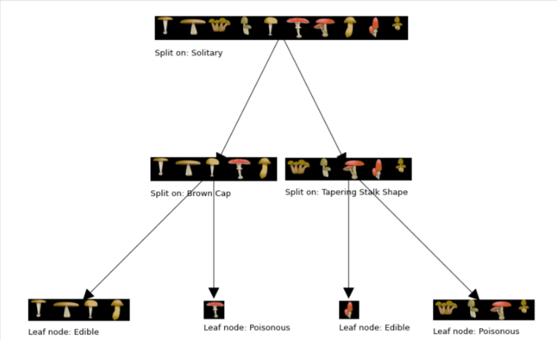
Build Tree

Build the tree by successively picking the best feature to split on, until we reach the stopping criteria being maximum depth = 2

tree = []

def build_tree_recursive(X, y, node_indices, branch_name, max_depth, current_depth):
    """
    Build a tree using the recursive algorithm that split the dataset into 2 subgroups at each node.
    This function just prints the tree.
    
    Args:
        X (ndarray):            Data matrix of shape(n_samples, n_features)
        y (array like):         list or ndarray with n_samples containing the target variable
        node_indices (ndarray): List containing the active indices. I.e, the samples being considered in this step.
        branch_name (string):   Name of the branch. ['Root', 'Left', 'Right']
        max_depth (int):        Max depth of the resulting tree. 
        current_depth (int):    Current depth. Parameter used during recursive call.
   
    """ 

    # Maximum depth reached - stop splitting
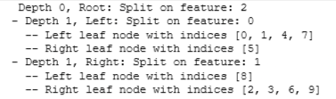
    if current_depth == max_depth:
        formatting = " "*current_depth + "-"*current_depth
        print(formatting, "%s leaf node with indices" % branch_name, node_indices)
        return
   
    # Otherwise, get best split and split the data
    # Get the best feature and threshold at this node
    best_feature = get_best_split(X, y, node_indices) 
    
    formatting = "-"*current_depth
    print("%s Depth %d, %s: Split on feature: %d" % (formatting, current_depth, branch_name, best_feature))
    
    # Split the dataset at the best feature
    left_indices, right_indices = split_dataset(X, node_indices, best_feature)
    tree.append((left_indices, right_indices, best_feature))
    
    # continue splitting the left and the right child. Increment current depth
    build_tree_recursive(X, y, left_indices, "Left", max_depth, current_depth+1)
    build_tree_recursive(X, y, right_indices, "Right", max_depth, current_depth+1)

build_tree_recursive(X_train, y_train, root_indices, "Root", max_depth=2, current_depth=0)
generate_tree_viz(root_indices, y_train, tree)