import copy, math
import numpy as np
import matplotlib.pyplot as plt
plt.style.use('./deeplearning.mplstyle')
np.set_printoptions(precision=2) # reduced display precision on numpy arraysGradient Descent
My thanks and credit to Stanford University & Andrew Ng for their contributions.
Single Variable LR
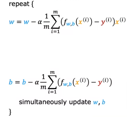
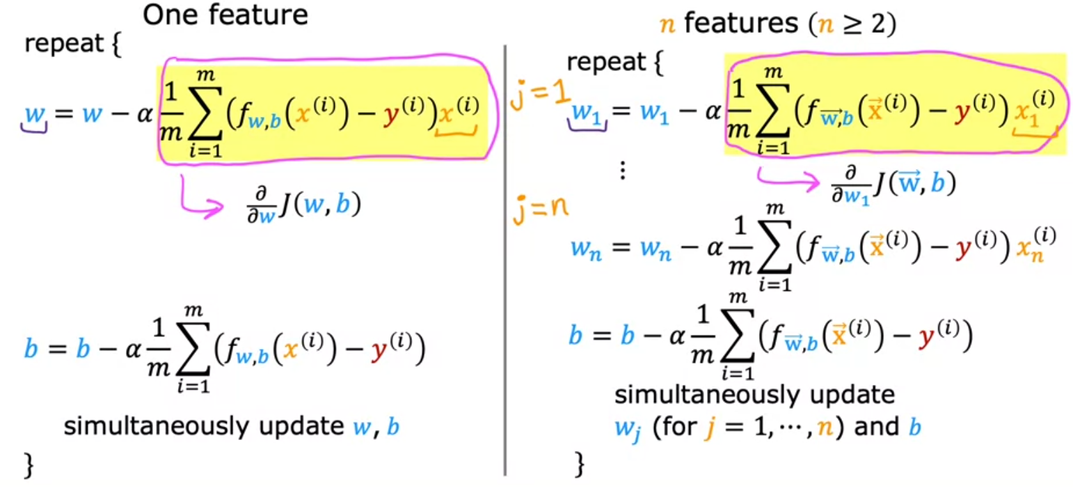
To summarize how we got here, remember for single variable LR model, cost and gradient descent are:
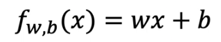
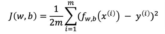
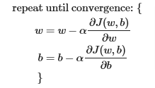
or can put like this:
Multiple Variable LR
Here are the formula starting with Gradient Descent first compared to single variable above
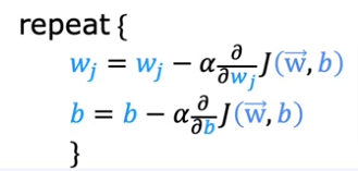

- n is the number of features
- wj and b are updated simultaneously
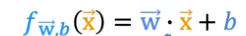
- w and x are vectors not a scalar
- m is the number of training examples in the data set
- fw,b(x(i)) is the model’s prediction, while y(i) is the target value
In totality compared to the One feature formulas
Alternative
If you want to use another method aside from GD ONLY on single variable LR, and only on LR you can use Normal Equation which is solved without w, b without iterations. It is slow when number of features is large >1000
Code
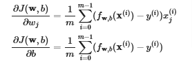
Calculate Gradient
Let’s first calculate the gradient which is shown in the image below
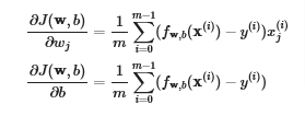
- outer loop over all m examples.
∂J(w,b)∂b for the example can be computed directly and accumulated
in a second loop over all n features:
- ∂J(w,b)∂wj is computed for each wj.
X_train = np.array([[2104, 5, 1, 45], [1416, 3, 2, 40], [852, 2, 1, 35]])
y_train = np.array([460, 232, 178])
b_init = 785.1811367994083
w_init = np.array([ 0.39133535, 18.75376741, -53.36032453, -26.42131618])
print(f"w_init shape: {w_init.shape}, b_init type: {type(b_init)}")w_init shape: (4,), b_init type: <class 'float'>def compute_gradient(X, y, w, b):
"""
Computes the gradient for linear regression
Args:
X (ndarray (m,n)): Data, m examples with n features
y (ndarray (m,)) : target values
w (ndarray (n,)) : model parameters
b (scalar) : model parameter
Returns:
dj_dw (ndarray (n,)): The gradient of the cost w.r.t. the parameters w.
dj_db (scalar): The gradient of the cost w.r.t. the parameter b.
"""
m,n = X.shape #(number of examples, number of features)
dj_dw = np.zeros((n,))
dj_db = 0.
for i in range(m):
err = (np.dot(X[i], w) + b) - y[i]
for j in range(n):
dj_dw[j] = dj_dw[j] + err * X[i, j]
dj_db = dj_db + err
dj_dw = dj_dw / m
dj_db = dj_db / m
return dj_db, dj_dw#Compute and display gradient
tmp_dj_db, tmp_dj_dw = compute_gradient(X_train, y_train, w_init, b_init)
print(f'dj_db at initial w,b: {tmp_dj_db}')
print(f'dj_dw at initial w,b: \n {tmp_dj_dw}')dj_db at initial w,b: -1.6739251501955248e-06
dj_dw at initial w,b:
[-2.73e-03 -6.27e-06 -2.22e-06 -6.92e-05].
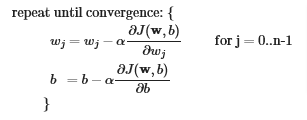
Calculate G Descent
Now let’s calculate the gradient descent using the values from compute_gradient, as well as compute_cost which I show below (was covered in previous page), as shown in the image below
def compute_cost(X, y, w, b):
    """
    compute cost
    Args:
      X (ndarray (m,n)): Data, m examples with n features
      y (ndarray (m,)) : target values
      w (ndarray (n,)) : model parameters
      b (scalar)       : model parameter

    Returns:
      cost (scalar): cost
    """
    m = X.shape[0]
    cost = 0.0
    for i in range(m):
        f_wb_i = np.dot(X[i], w) + b           #(n,)(n,) = scalar (see np.dot)
        cost = cost + (f_wb_i - y[i])**2       #scalar
    cost = cost / (2 * m)                      #scalar
    return cost
def gradient_descent(X, y, w_in, b_in, cost_function, gradient_function, alpha, num_iters):
"""
Performs batch gradient descent to learn theta. Updates theta by taking
num_iters gradient steps with learning rate alpha
Args:
X (ndarray (m,n)) : Data, m examples with n features
y (ndarray (m,)) : target values
w_in (ndarray (n,)) : initial model parameters
b_in (scalar) : initial model parameter
cost_function : function to compute cost
gradient_function : function to compute the gradient
alpha (float) : Learning rate
num_iters (int) : number of iterations to run gradient descent
Returns:
w (ndarray (n,)) : Updated values of parameters
b (scalar) : Updated value of parameter
"""
# An array to store cost J and w's at each iteration primarily for graphing later
J_history = []
w = copy.deepcopy(w_in) #avoid modifying global w within function
b = b_in
for i in range(num_iters):
# Calculate the gradient and update the parameters
dj_db,dj_dw = gradient_function(X, y, w, b) ##None
# Update Parameters using w, b, alpha and gradient
w = w - alpha * dj_dw ##None
b = b - alpha * dj_db ##None
# Save cost J at each iteration
if i<100000: # prevent resource exhaustion
J_history.append( cost_function(X, y, w, b))
# Print cost every at intervals 10 times or as many iterations if < 10
if i% math.ceil(num_iters / 10) == 0:
print(f"Iteration {i:4d}: Cost {J_history[-1]:8.2f} ")
return w, b, J_history #return final w,b and J history for graphingCall Functions
# initialize parameters
initial_w = np.zeros_like(w_init)
initial_b = 0.
# some gradient descent settings
iterations = 1000
alpha = 5.0e-7
# run gradient descent
w_final, b_final, J_hist = gradient_descent(X_train, y_train, initial_w, initial_b,
                                                    compute_cost, compute_gradient,
                                                    alpha, iterations)
print(f"b,w found by gradient descent: {b_final:0.2f},{w_final} ")
m,_ = X_train.shape
for i in range(m):
    print(f"prediction: {np.dot(X_train[i], w_final) + b_final:0.2f}, target value: {y_train[i]}")
Iteration 0: Cost 2529.46
Iteration 100: Cost 695.99
Iteration 200: Cost 694.92
Iteration 300: Cost 693.86
Iteration 400: Cost 692.81
Iteration 500: Cost 691.77
Iteration 600: Cost 690.73
Iteration 700: Cost 689.71
Iteration 800: Cost 688.70
Iteration 900: Cost 687.69
b,w found by gradient descent: -0.00,[ 0.2 0. -0.01 -0.07]
prediction: 426.19, target value: 460
prediction: 286.17, target value: 232
prediction: 171.47, target value: 178Plot
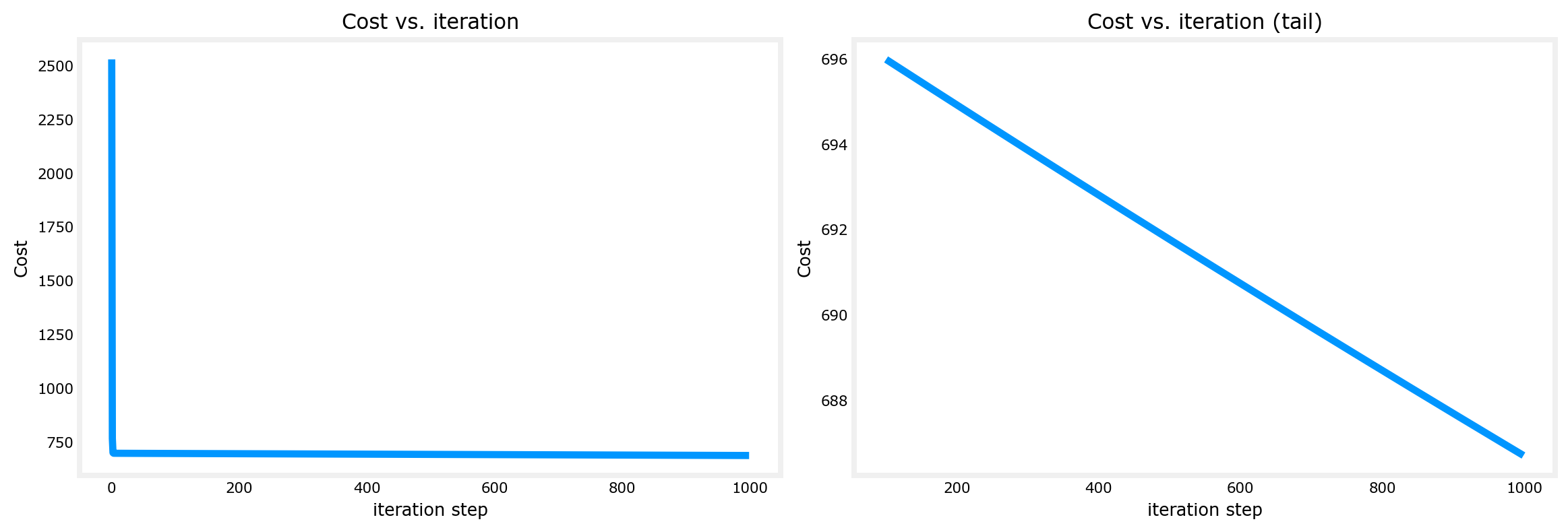
Let’s plot cost vs iterations
- As we see, cost is still declining and our predictions are not very accurate
# plot cost versus iteration
fig, (ax1, ax2) = plt.subplots(1, 2, constrained_layout=True, figsize=(12, 4))
ax1.plot(J_hist)
ax2.plot(100 + np.arange(len(J_hist[100:])), J_hist[100:])
ax1.set_title("Cost vs. iteration");  ax2.set_title("Cost vs. iteration (tail)")
ax1.set_ylabel('Cost')             ;  ax2.set_ylabel('Cost')
ax1.set_xlabel('iteration step')   ;  ax2.set_xlabel('iteration step')
plt.show()