# All Libraries required for this lab are listed below. Already installed so this code block is commented out
pip install pandas==1.3.4
pip install scikit-learn==1.0.2Build & Evaluate Classifier for Diabetes
Objectives
We will use iris dataset to create a classifier then evaluate it using various metrics
Here is a list of Tasks we’ll be doing:
- Use Pandas to load data sets.
- Identify the target and features.
- Use Logistic Regression to build a classifier.
- Use metrics to evaluate the model.
- Make predictions using a trained model.
Setup
We will be using the following libraries:
pandasfor managing the data.sklearnfor machine learning and machine-learning-pipeline related functions.
Install Libraries
Suppress Warnings
To suppress warnings generated by our code, we’ll use this code block
# To suppress warnings generated by the code
def warn(*args, **kwargs):
    pass
import warnings
warnings.warn = warn
warnings.filterwarnings('ignore')
Import Libraries
import pandas as pd
from sklearn.linear_model import LogisticRegression

#import functions for train test split
from sklearn.model_selection import train_test_split


# functions for metrics

from sklearn.metrics import confusion_matrix
from sklearn.metrics import precision_score
from sklearn.metrics import recall_score
from sklearn.metrics import f1_score
Data - Task 1
- Modified version of Pima Indians Diabetes Database. Available at https://www.kaggle.com/datasets/uciml/pima-indians-diabetes-database
Load
# the data set is available at the url below.
URL = "https://cf-courses-data.s3.us.cloud-object-storage.appdomain.cloud/IBM-BD0231EN-SkillsNetwork/datasets/diabetes.csv"

# using the read_csv function in the pandas library, we load the data into a dataframe
df = pd.read_csv(URL)
# you can sample the data with df.sample(5)|
|
|
Glucose |
BloodPressure |
SkinThickness |
Insulin |
BMI |
DiabetesPedigreeFunction |
Age |
Outcome |
|---|---|---|---|---|---|---|---|---|---|
|
145 |
0 |
102 |
75 |
23 |
0 |
0.0 |
0.572 |
21 |
0 |
|
470 |
1 |
144 |
82 |
40 |
0 |
41.3 |
0.607 |
28 |
0 |
|
142 |
2 |
108 |
52 |
26 |
63 |
32.5 |
0.318 |
22 |
0 |
|
633 |
1 |
128 |
82 |
17 |
183 |
27.5 |
0.115 |
22 |
0 |
|
150 |
1 |
136 |
74 |
50 |
204 |
37.4 |
0.399 |
24 |
0 |
df.shape(768, 9)Plot Data
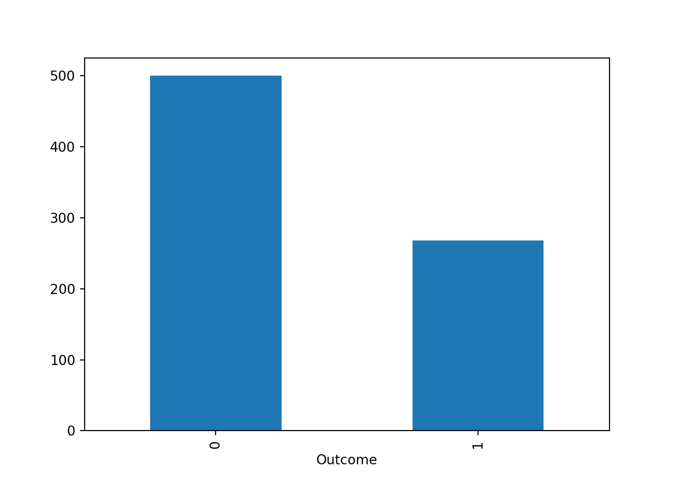
- Let’s plot the types and count of Outcome
- There are 500 people without diabetes and 268 people with diabetes in this dataset.
df.Outcome.value_counts()Outcome
0 500
1 268
Name: count, dtype: int64df.Outcome.value_counts().plot.bar()
Define Targets/Features - Task 2
Target
In Classification models, the Target (Y) is the value our machine learning model needs to classify
So, in this example we are trying to classify the Outcome
Features
The feature(s) is/are the data columns we will provide our model as input from which our model learns from
In our example let’s provide the model with these Features, and see how accurate it will be in predicting the list is in the code
# Target is our Y
Y = df["Outcome"]

# Features is our X
X = df[['Pregnancies', 'Glucose', 'BloodPressure', 'SkinThickness', 'Insulin',
       'BMI', 'DiabetesPedigreeFunction', 'Age']]
Split Dataset - Task 3
- We now split the data at 70/30 ratio, 70 training, 30 testing
- The random_state variable controls the shuffling applied to the data before applying the split.
- Pass the same integer for reproducible output across multiple function calls
X_train, X_test, Y_train, Y_test = train_test_split(X, Y, test_size=0.30, random_state=40)Build & Train Classifier - Task 4
Logistic Regression Model
Create a Logistic Regression model
classifier = LogisticRegression()Train Logistic Regression Model
Response will be:
- LogisticRegression(C=1.0, class_weight=None, dual=False, fit_intercept=True, intercept_scaling=1, max_iter=100, multi_class=‘warn’, n_jobs=None, penalty=‘l2’, random_state=None, solver=‘warn’, tol=0.0001, verbose=0, warm_start=False)
classifier.fit(X_train, Y_train)LogisticRegression()In a Jupyter environment, please rerun this cell to show the HTML representation or trust the notebook.
On GitHub, the HTML representation is unable to render, please try loading this page with nbviewer.org.
LogisticRegression()
Evaluate Model - Task 5
Now that the model has been trained on the data/features provided above, let’s evaluate it
Score
The higher the better
#Higher the score, better the model.
classifier.score(X_test, Y_test)0.7229437229437229Predict
In order to calculate the score metrics we need two values:
- The original values from the test data set and we’ll compare to the predicted values
- The predicted values which are the results of the model
original_values = Y_test
predicted_values = classifier.predict(X_test)
Precision
The higher the value the better the model
precision_score(original_values, predicted_values)0.6865671641791045Recall
The higher the value the better the model
recall_score(original_values, predicted_values)0.5168539325842697F1 Score
The higher the value the better the model
f1_score(original_values, predicted_values)0.5897435897435898Confusion Matrix
This can be used to manually calculate various metrics
confusion_matrix(original_values, predicted_values)array([[121, 21],
[ 43, 46]])