import numpy as np
import matplotlib.pyplot as plt
from utils import *
import copy
import math
#%matplotlib inlineLR Predict Profit
Case Study
Suppose you are considering different cities for opening a new outlet.
- You would like to expand your business to cities that may give your restaurant higher profits.
- The chain already has restaurants in various cities and you have data for profits and populations from the cities.
- You also have data on cities that are candidates for a new restaurant.
- For these cities, you have the city population.
Can you use the data to help you identify which cities may potentially give your business higher profits?
Setup
.
Dataset
The load_data() function shown below loads the data into variables x_train and y_train
def load_data():
    data = np.loadtxt("data/ex1data1.txt", delimiter=',')
    X = data[:,0]  # all of column 1
    y = data[:,1]  # all of column 2
return X, yx_trainis the population of a cityy_trainis the profit of a restaurant in that city. A negative value for profit indicates a loss.- Both
X_trainandy_trainare numpy arrays. - Data is in ex1data1.txt
# load the dataset
x_train, y_train = load_data()
View Data
Let’s see the x_train data:
x_train is a numpy array that contains decimal values that are all greater than zero.
- These values represent the city population times 10,000
- For example, 6.1101 means that the population for that city is 61,101
# print x_train
print("Type of x_train:",type(x_train))
print("First five elements of x_train are:\n", x_train[:5]) 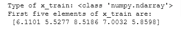
Let’s see the y_train data:
Similarly, y_train is a numpy array that has decimal values, some negative, some positive.
These represent your restaurant’s average monthly profits in each city, in units of $10,000.
- For example, 17.592 represents $175,920 in average monthly profits for that city.
- -2.6807 represents -$26,807 in average monthly loss for that city.
# print y_train
print("Type of y_train:",type(y_train))
print("First five elements of y_train are:\n", y_train[:5]) 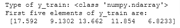
View Dimensions
Let’s look at the dimensions of our variables:
- The city population array has 97 data points, and the monthly average profits also has 97 data points. Both are NumPy 1D arrays
print ('The shape of x_train is:', x_train.shape)
print ('The shape of y_train is: ', y_train.shape)
print ('Number of training examples (m):', len(x_train))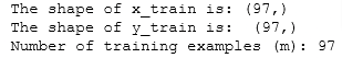
View Data
- For this dataset, you can use a scatter plot to visualize the data, since it has only two properties to plot (profit and population).
- Many other problems that you will encounter in real life have more than two properties (for example, population, average household income, monthly profits, monthly sales).When you have more than two properties, you can still use a scatter plot to see the relationship between each pair of properties.
# Create a scatter plot of the data. To change the markers to red "x",
# we used the 'marker' and 'c' parameters
#v = x_train[:,0]

plt.scatter(x_train, y_train, marker='x', c='r')

# Set the title
plt.title("Profits vs. Population per city")
# Set the y-axis label
plt.ylabel('Profit in $10,000')
# Set the x-axis label
plt.xlabel('Population of City in 10,000s')
plt.show()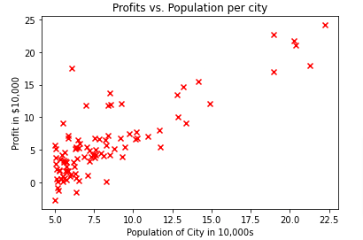
Now we can build a linear regression model to fit this data. Now we can input a new city population and have the model estimate your restaurant’s potential profits
LR Model
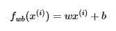
So the model maps from x (city population) to y (monthly profit) is represented as
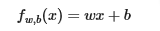
- We want to train our LR model to find the best (w,b) parameters that fit the dataset
- We will use the cost function J(w,b) to decide which values to use for those parameters
- The best values are the ones that have the smallest cost J(w,b)
Compute Cost
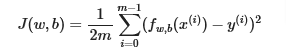
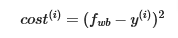
- You can think of fw,b(x(i)) as the model’s prediction of your restaurant’s profit, as opposed to y(i), which is the actual profit that is recorded in the data.
- m is the number of training examples in the dataset
- So the model prediction is with a line with an intercept at b and a slope w
- So let’s compute the cost first
- Return the total cost over all examples with m being the number of training examples summed over all examples
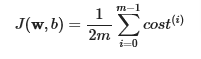
- Let’s create a function that calculates the cost J(w,b) and name it compute_cost
# Compute_cost function
def compute_cost(x, y, w, b):
    """
    Computes the cost function for linear regression.

    Args:
        x (ndarray): Shape (m,) Input to the model (Population of cities)
        y (ndarray): Shape (m,) Label (Actual profits for the cities)
        w, b (scalar): Parameters of the model

    Returns
        total_cost (float): The cost of using w,b as the parameters for linear regression
               to fit the data points in x and y
    """
    # number of training examples
    m = x.shape[0]

    # You need to return this variable correctly
    total_cost = 0

    # Variable to keep track of sum of cost from each example
    cost_sum = 0

    # Loop over training examples
    for i in range(m):
        # Your code here to get the prediction f_wb for the ith example
        f_wb = w * x[i] + b
        # Your code here to get the cost associated with the ith example
        cost = (f_wb - y[i]) ** 2

        # Add to sum of cost for each example
        cost_sum = cost_sum + cost

    # Get the total cost as the sum divided by (2*m)
    total_cost = (1 / (2 * m)) * cost_sum

    return total_cost
View Cost
# Compute cost with some initial values for paramaters w, b
initial_w = 2
initial_b = 1

cost = compute_cost(x_train, y_train, initial_w, initial_b)
print(type(cost))
print(f'Cost at initial w: {cost:.3f}')

# Public tests
from public_tests import *
compute_cost_test(compute_cost)
Calculate Gradient
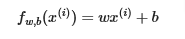
Let’s implement the gradient descent using parameters w and b for LR. Let’s create a function named compute_gradient which
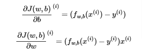
- Iterates over the training example, and for each example, compute:
- The prediction model for that example, described as
- The gradient for the parameters b and w from that example is
- The gradient descent algorithm is
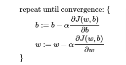
- parameters w and b are both updated simultaneously
- m is the number of training examples in the dataset
- fw,b(x(i)) is the model’s prediction, while u(i) is the target value
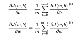
- return the total gradient update from all the examples
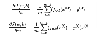
- which is the same as
# compute_gradient
def compute_gradient(x, y, w, b):
    """
    Computes the gradient for linear regression
    Args:
      x (ndarray): Shape (m,) Input to the model (Population of cities)
      y (ndarray): Shape (m,) Label (Actual profits for the cities)
      w, b (scalar): Parameters of the model
    Returns
      dj_dw (scalar): The gradient of the cost w.r.t. the parameters w
      dj_db (scalar): The gradient of the cost w.r.t. the parameter b
     """

    # Number of training examples
    m = x.shape[0]

    # You need to return the following variables correctly
    dj_dw = 0
    dj_db = 0

    for i in range(m):
        # Predict f_wb for the ith example
        f_wb = w * x[i] + b

        # Get the gradient for w from the ith example
        dj_dw_i = (f_wb - y[i]) * x[i]

        # Get the gradient for b from the ith example
        dj_db_i = f_wb - y[i]

        # Update dj_db: remember x += 1 is equivalent to x = x + 1
        dj_db += dj_db_i

        # Update dj_dw
        dj_dw += dj_dw_i

    # Divide both dj_dw and dj_db by m
    dj_dw = dj_dw / m
    dj_db = dj_db / m

    return dj_dw, dj_db
View Gradient
With w and b set to 0
# Compute and display gradient with w initialized to zeroes
initial_w = 0
initial_b = 0

tmp_dj_dw, tmp_dj_db = compute_gradient(x_train, y_train, initial_w, initial_b)
print('Gradient at initial w, b (zeros):', tmp_dj_dw, tmp_dj_db)

compute_gradient_test(compute_gradient)
With w and b non-zero
# Compute and display cost and gradient with non-zero w
test_w = 0.2
test_b = 0.2
tmp_dj_dw, tmp_dj_db = compute_gradient(x_train, y_train, test_w, test_b)

print('Gradient at test w, b:', tmp_dj_dw, tmp_dj_db)
Batch Gradient Descent
Using Batch Gradient Descent, we will now find the optimal parameters of a linear regression model by using batch gradient descent. Recall batch refers to running all the examples in one iteration.
A good way to verify that gradient descent is working correctly is to look at the value of J(w,b) and check that it is decreasing with each step.
Assuming we have implemented the gradient and computed the cost correctly and we have an appropriate value for the learning rate alpha, J(w,b) should never increase and should converge to a steady value by the end of the algorithm.
Create Gradient Descent Function named gradient_descent
Note the cost_function and gradient_function are not the ones described above as obviously are named differently, but you can substitute your functions
def gradient_descent(x, y, w_in, b_in, cost_function, gradient_function, alpha, num_iters):
    """
    Performs batch gradient descent to learn theta. Updates theta by taking
    num_iters gradient steps with learning rate alpha

    Args:
      x :    (ndarray): Shape (m,)
      y :    (ndarray): Shape (m,)
      w_in, b_in : (scalar) Initial values of parameters of the model
      cost_function: function to compute cost
      gradient_function: function to compute the gradient
      alpha : (float) Learning rate
      num_iters : (int) number of iterations to run gradient descent
    Returns
      w : (ndarray): Shape (1,) Updated values of parameters of the model after
          running gradient descent
      b : (scalar)                Updated value of parameter of the model after
          running gradient descent
    """

    # number of training examples
    m = len(x)

    # An array to store cost J and w's at each iteration — primarily for graphing later
    J_history = []
    w_history = []
    w = copy.deepcopy(w_in)  #avoid modifying global w within function
    b = b_in

    for i in range(num_iters):

        # Calculate the gradient and update the parameters
        dj_dw, dj_db = gradient_function(x, y, w, b )

        # Update Parameters using w, b, alpha and gradient
        w = w - alpha * dj_dw
        b = b - alpha * dj_db

        # Save cost J at each iteration
        if i<100000:      # prevent resource exhaustion
            cost =  cost_function(x, y, w, b)
            J_history.append(cost)

        # Print cost every at intervals 10 times or as many iterations if < 10
        if i% math.ceil(num_iters/10) == 0:
            w_history.append(w)
            print(f"Iteration {i:4}: Cost {float(J_history[-1]):8.2f}   ")

    return w, b, J_history, w_history #return w and J,w history for graphing
View GD
# initialize fitting parameters. Recall that the shape of w is (n,)
initial_w = 0.
initial_b = 0.

# some gradient descent settings
iterations = 1500
alpha = 0.01

w,b,_,_ = gradient_descent(x_train ,y_train, initial_w, initial_b,
                     compute_cost, compute_gradient, alpha, iterations)
print("w,b found by gradient descent:", w, b)
Plot Linear Fit
We will now use the final parameters from gradient descent to plot the linear fit. Recall that we can get the prediction for a single example f(x(i))=wx(i)+b.
To calculate the predictions on the entire dataset, we can loop through all the training examples and calculate the prediction for each example. This is shown in the code block below.
m = x_train.shape[0]
predicted = np.zeros(m)

for i in range(m):
    predicted[i] = w * x_train[i] + b
Let’s plot it
# Plot the linear fit
plt.plot(x_train, predicted, c = "b")

# Create a scatter plot of the data.
plt.scatter(x_train, y_train, marker='x', c='r')

# Set the title
plt.title("Profits vs. Population per city")
# Set the y-axis label
plt.ylabel('Profit in $10,000')
# Set the x-axis label
plt.xlabel('Population of City in 10,000s')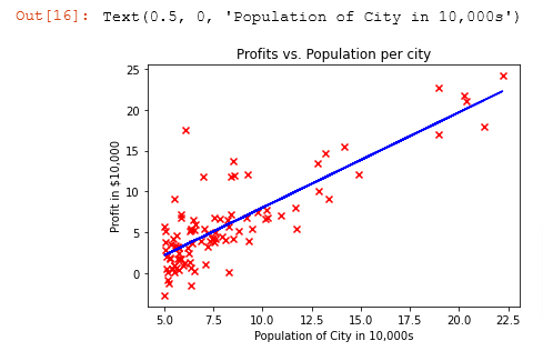
Predictions
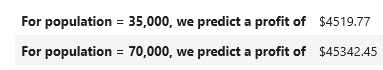
Our final values of w,b can also be used to make predictions on profits. Let’s predict what the profit would be in areas of 35,000 and 70,000 people.
- The model takes in population of a city in 10,000s as input.
- Therefore, 35,000 people can be translated into an input to the model as
np.array([3.5]) - Similarly, 70,000 people can be translated into an input to the model as
np.array([7.])
predict1 = 3.5 * w + b
print('For population = 35,000, we predict a profit of $%.2f' % (predict1*10000))

predict2 = 7.0 * w + b
print('For population = 70,000, we predict a profit of $%.2f' % (predict2*10000))