import numpy as np
#%matplotlib widget
import matplotlib.pyplot as plt
#from plt_one_addpt_onclick import plt_one_addpt_onclick
#from lab_utils_common import draw_vthresh
plt.style.use('./deeplearning.mplstyle')
import copy
import math
import matplotlib.pyplot as plt
from matplotlib.patches import FancyArrowPatch
#from ipywidgets import OutputSigmoid Function
Logistic Regression
Since LR algorithms are not ideal for classification problems we will go through one of the most popular algorithms for it. Logistic Regression. We’ll cover the separate parts that make up the model:
.
Sigmoid Function
As discussed earlier, for a classification task, we can start by using our linear regression model, fw,b(x(i))=w⋅x(i)+b, to predict y given x.
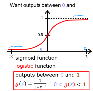
- However, we would like the predictions of our classification model to be between 0 and 1 since our output variable y is either 0 or 1.
- This can be accomplished by using a “sigmoid function” which maps all input values to values between 0 and 1.
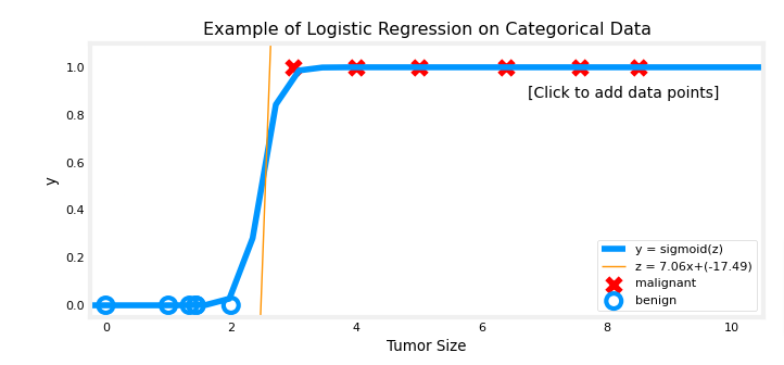
- So is we want to classify if a tumor is malignant or not
- The logistic regression curve will look like the image below
Let’s implement the sigmoid/logistic function and see this for ourselves.
Formula
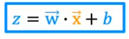
- The input to the Sigmoid Function g((z), is the output of the Linear Regression model. So if you remember the linear algorithm is
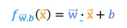
- So the output of the linear regression formula is the input of the Sigmoid Function g(z)
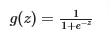
- So the formula for g(z) will be
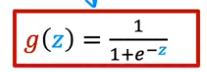
- Numpy can be used for the exponential function: exp()
- The formula will water down to
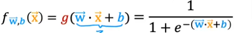
- If we are dealing with a single example, z is scalar
- In the event of multiple examples, z may be a vector consistent of m values one for each example
- So to cover all cases, the formula should cover both of these potential input formats
- What you also notice is that the vertical axis is centered at z and z values are symmetrical on both + and - axis
- So as you see when z is very large the g(z) will become very close to 1 and when z is very large negative number it will approach 0
- If z =0 then the formula will give us: g(z) = 1/2 = 0.5
Output
Think of the logistic regression output as the probability that the output of y is % of being 1
So if x is tumor size and y =0 (not malignant) and y=1 (malignant), then fw,b(x) = 0.7 means that we have a 70% chance that y is 1
So if the probability of it being 1 is 0.7 it means that the probability of it being 0 is 0.3 because the formula is:
P(y=0) - P(y=1) = 1
Code
Setup
Since we know that we can calculate the exponential function using Numpy, then the Sigmoid function is implemented like this
def sigmoid(z):
    """
    Compute the sigmoid of z

    Args:
        z (ndarray): A scalar, numpy array of any size.

    Returns:
        g (ndarray): sigmoid(z), with the same shape as z

    """

    g = 1/(1+np.exp(-z))

    return g
Threshold Function
def draw_vthresh(ax,x):
    """ draws a threshold """
    dlc = dict(dlblue = '#0096ff', dlorange = '#FF9300', dldarkred='#C00000', dlmagenta='#FF40FF', dlpurple='#7030A0')
    dlblue = '#0096ff'; dlorange = '#FF9300'; dldarkred='#C00000'; dlmagenta='#FF40FF'; dlpurple='#7030A0'
    dlcolors = [dlblue, dlorange, dldarkred, dlmagenta, dlpurple]
    ylim = ax.get_ylim()
    xlim = ax.get_xlim()
    ax.fill_between([xlim[0], x], [ylim[1], ylim[1]], alpha=0.2, color=dlblue)
    ax.fill_between([x, xlim[1]], [ylim[1], ylim[1]], alpha=0.2, color=dldarkred)
    ax.annotate("z >= 0", xy= [x,0.5], xycoords='data',
                xytext=[30,5],textcoords='offset points')
    d = FancyArrowPatch(
        posA=(x, 0.5), posB=(x+3, 0.5), color=dldarkred,
        arrowstyle='simple, head_width=5, head_length=10, tail_width=0.0',
    )
    ax.add_artist(d)
    ax.annotate("z < 0", xy= [x,0.5], xycoords='data',
                 xytext=[-50,5],textcoords='offset points', ha='left')
    f = FancyArrowPatch(
        posA=(x, 0.5), posB=(x-3, 0.5), color=dlblue,
        arrowstyle='simple, head_width=5, head_length=10, tail_width=0.0',
    )
    ax.add_artist(f)
Data
- Let’s generate an array of evenly spaced values between -10 & 10
- Calculate the sigmoid value for each
- Plot the sigmoid curve
- You can see in the printout that the value of g() varies from 0 to 1
# Generate an array of evenly spaced values between -10 and 10
z_tmp = np.arange(-10,11)

# Use the function implemented above to get the sigmoid values
y = sigmoid(z_tmp)

# Code for pretty printing the two arrays next to each other
np.set_printoptions(precision=3)
print("Input (z), Output (sigmoid(z))")
print(np.c_[z_tmp, y])
Input (z), Output (sigmoid(z))
[[-1.000e+01 4.540e-05]
[-9.000e+00 1.234e-04]
[-8.000e+00 3.354e-04]
[-7.000e+00 9.111e-04]
[-6.000e+00 2.473e-03]
[-5.000e+00 6.693e-03]
[-4.000e+00 1.799e-02]
[-3.000e+00 4.743e-02]
[-2.000e+00 1.192e-01]
[-1.000e+00 2.689e-01]
[ 0.000e+00 5.000e-01]
[ 1.000e+00 7.311e-01]
[ 2.000e+00 8.808e-01]
[ 3.000e+00 9.526e-01]
[ 4.000e+00 9.820e-01]
[ 5.000e+00 9.933e-01]
[ 6.000e+00 9.975e-01]
[ 7.000e+00 9.991e-01]
[ 8.000e+00 9.997e-01]
[ 9.000e+00 9.999e-01]
[ 1.000e+01 1.000e+00]]# Plot z vs sigmoid(z)
fig,ax = plt.subplots(1,1,figsize=(5,3))
ax.plot(z_tmp, y, c="b")
ax.set_title("Sigmoid function")
ax.set_ylabel('sigmoid(z)')
ax.set_xlabel('z')
draw_vthresh(ax,0)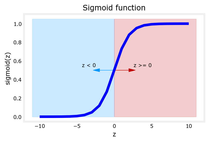
Logistic Regression
- Let’s apply logistic regression to the categorical data exmaple of tumor classifications
- Load the data
- Use function in python file to plot
x_train = np.array([0., 1, 2, 3, 4, 5])
y_train = np.array([0,  0, 0, 1, 1, 1])

w_in = np.zeros((1))
b_in = 0plt.close('all')
addpt = plt_one_addpt_onclick( x_train,y_train, w_in, b_in, logistic=True)