# for array computations and loading data
import numpy as np

# for building linear regression models and preparing data
from sklearn.linear_model import LinearRegression
from sklearn.preprocessing import StandardScaler, PolynomialFeatures
from sklearn.model_selection import train_test_split
from sklearn.metrics import mean_squared_error

# for building and training neural networks
import tensorflow as tf

# custom functions
import utils

# reduce display precision on numpy arrays
np.set_printoptions(precision=2)

# suppress warnings
tf.get_logger().setLevel('ERROR')
tf.autograph.set_verbosity(0)Tips for ML
Quantifying a learning algorithm’s performance and comparing different models are some of the common tasks when applying machine learning to real world applications.
Evaluation
.
Regression Model
Develop a model for regression problem given a dataset of 50 examples of an input feature x and its corresponding target y.
# Load the dataset from the text file
data = np.loadtxt('./data/data_w3_ex1.csv', delimiter=',')

# Split the inputs and outputs into separate arrays
x = data[:,0]
y = data[:,1]

# Convert 1-D arrays into 2-D because the commands later will require it
x = np.expand_dims(x, axis=1)
y = np.expand_dims(y, axis=1)

print(f"the shape of the inputs x is: {x.shape}")
print(f"the shape of the targets y is: {y.shape}")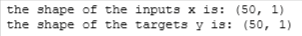
# Plot the entire dataset
utils.plot_dataset(x=x, y=y, title="input vs. target")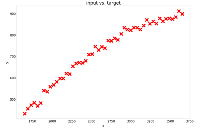
Split Data
Split into Training, cross validation, and test sets
- training set - used to train the model
- cross validation set (also called validation, development, or dev set) - used to evaluate the different model configurations you are choosing from. For example, you can use this to make a decision on what polynomial features to add to your dataset.
- test set - used to give a fair estimate of your chosen model’s performance against new examples. This should not be used to make decisions while you are still developing the models.
Scikit-learn provides a train_test_split function to split your data into the parts mentioned above. In the code cell below, you will split the entire dataset into 60% training, 20% cross validation, and 20% test.
# Get 60% of the dataset as the training set. Put the remaining 40% in temporary variables: x_ and y_.
x_train, x_, y_train, y_ = train_test_split(x, y, test_size=0.40, random_state=1)

# Split the 40% subset above into two: one half for cross validation and the other for the test set
x_cv, x_test, y_cv, y_test = train_test_split(x_, y_, test_size=0.50, random_state=1)

# Delete temporary variables
del x_, y_

print(f"the shape of the training set (input) is: {x_train.shape}")
print(f"the shape of the training set (target) is: {y_train.shape}\n")
print(f"the shape of the cross validation set (input) is: {x_cv.shape}")
print(f"the shape of the cross validation set (target) is: {y_cv.shape}\n")
print(f"the shape of the test set (input) is: {x_test.shape}")
print(f"the shape of the test set (target) is: {y_test.shape}")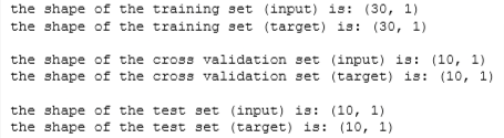
Let’s see which points were used as training, cross validation, or test data
utils.plot_train_cv_test(x_train, y_train, x_cv, y_cv, x_test, y_test, title="input vs. target")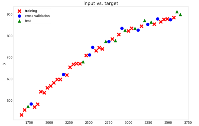
Scale Features
Use the StandardScaler class from scikit-learn. This computes the z-score of your inputs. As a refresher, the z-score is given by the equation:

x.# Initialize the class
scaler_linear = StandardScaler()
# Compute the mean and standard deviation of the training set then transform it
X_train_scaled = scaler_linear.fit_transform(x_train)
print(f"Computed mean of the training set: {scaler_linear.mean_.squeeze():.2f}")
print(f"Computed standard deviation of the training set: {scaler_linear.scale_.squeeze():.2f}")
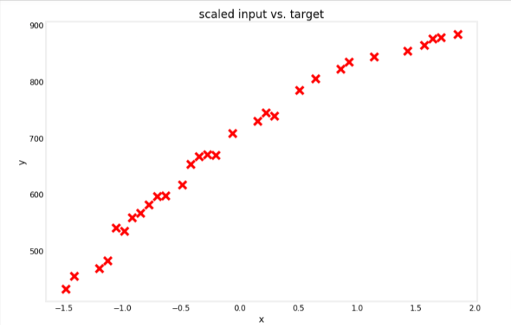
# Plot the results
utils.plot_dataset(x=X_train_scaled, y=y_train, title="scaled input vs. target")
Train Model
We will use a linear model
# Initialize the class
linear_model = LinearRegression()

# Train the model
linear_model.fit(X_train_scaled, y_train )
Evaluate Model
MSE Training Set
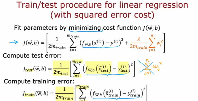
To evaluate the performance of your model, you will measure the error for the training and cross validation sets. For the training error, recall the equation for calculating the mean squared error (MSE):
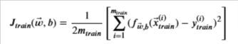
Scikit-learn also has a built-in mean_squared_error() function that you can use. Take note though that as per the documentation, scikit-learn’s implementation only divides by m and not 2*m, where m is the number of examples. As mentioned in Course 1 of this Specialization (cost function lectures), dividing by 2m is a convention we will follow but the calculations should still work whether or not you include it. Thus, to match the equation above, you can use the scikit-learn function then divide by 2 as shown below. We also included a for-loop implementation so you can check that it’s equal.
Another thing to take note: Since you trained the model on scaled values (i.e. using the z-score), you should also feed in the scaled training set instead of its raw values.
# Feed the scaled training set and get the predictions
yhat = linear_model.predict(X_train_scaled)

# Use scikit-learn's utility function and divide by 2
print(f"training MSE (using sklearn function): {mean_squared_error(y_train, yhat) / 2}")

# for-loop implementation
total_squared_error = 0

for i in range(len(yhat)):
    squared_error_i  = (yhat[i] - y_train[i])**2
    total_squared_error += squared_error_i

mse = total_squared_error / (2*len(yhat))

print(f"training MSE (for-loop implementation): {mse.squeeze()}")
MSE Xvalidation Set
As with the training set, you will also want to scale the cross validation set. An important thing to note when using the z-score is you have to use the mean and standard deviation of the training set when scaling the cross validation set. This is to ensure that your input features are transformed as expected by the model. One way to gain intuition is with this scenario:
- Say that your training set has an input feature equal to
500which is scaled down to0.5using the z-score. - After training, your model is able to accurately map this scaled input
x=0.5to the target outputy=300. - Now let’s say that you deployed this model and one of your users fed it a sample equal to
500. - If you get this input sample’s z-score using any other values of the mean and standard deviation, then it might not be scaled to
0.5and your model will most likely make a wrong prediction (i.e. not equal toy=300).
You will scale the cross validation set below by using the same StandardScaler you used earlier but only calling its transform() method instead of fit_transform().
# Scale the cross validation set using the mean and standard deviation of the training set
X_cv_scaled = scaler_linear.transform(x_cv)

print(f"Mean used to scale the CV set: {scaler_linear.mean_.squeeze():.2f}")
print(f"Standard deviation used to scale the CV set: {scaler_linear.scale_.squeeze():.2f}")

# Feed the scaled cross validation set
yhat = linear_model.predict(X_cv_scaled)

# Use scikit-learn's utility function and divide by 2
print(f"Cross validation MSE: {mean_squared_error(y_cv, yhat) / 2}")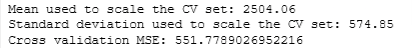
Add Features
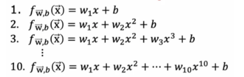
From the graphs earlier, you may have noticed that the target y rises more sharply at smaller values of x compared to higher ones. A straight line might not be the best choice because the target y seems to flatten out as x increases. Now that you have these values of the training and cross validation MSE from the linear model, you can try adding polynomial features to see if you can get a better performance. The code will mostly be the same but with a few extra preprocessing steps. Let’s see that below.
First, you will generate the polynomial features from your training set. The code below demonstrates how to do this using the PolynomialFeatures class. It will create a new input feature which has the squared values of the input x (i.e. degree=2).
# Instantiate the class to make polynomial features
poly = PolynomialFeatures(degree=2, include_bias=False)

# Compute the number of features and transform the training set
X_train_mapped = poly.fit_transform(x_train)

# Preview the first 5 elements of the new training set. Left column is `x` and right column is `x^2`
# Note: The `e+<number>` in the output denotes how many places the decimal point should
# be moved. For example, `3.24e+03` is equal to `3240`
print(X_train_mapped[:5])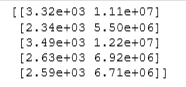
Scale Features
# Instantiate the class
scaler_poly = StandardScaler()

# Compute the mean and standard deviation of the training set then transform it
X_train_mapped_scaled = scaler_poly.fit_transform(X_train_mapped)

# Preview the first 5 elements of the scaled training set.
print(X_train_mapped_scaled[:5])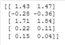
Train, Compare performance against the training results. Make sure to follow the same process as we did for the training set
# Initialize the class
model = LinearRegression()

# Train the model
model.fit(X_train_mapped_scaled, y_train )

# Compute the training MSE
yhat = model.predict(X_train_mapped_scaled)
print(f"Training MSE: {mean_squared_error(y_train, yhat) / 2}")

# Add the polynomial features to the cross validation set
X_cv_mapped = poly.transform(x_cv)

# Scale the cross validation set using the mean and standard deviation of the training set
X_cv_mapped_scaled = scaler_poly.transform(X_cv_mapped)

# Compute the cross validation MSE
yhat = model.predict(X_cv_mapped_scaled)
print(f"Cross validation MSE: {mean_squared_error(y_cv, yhat) / 2}")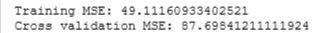
Add More Features
The MSEs are significantly better for both the training and cross validatioin set when the additional features were added. We can loop through and add more polynomial terms and see if the performance improves even more.
# Initialize lists to save the errors, models, and feature transforms
train_mses = []
cv_mses = []
models = []
polys = []
scalers = []

# Loop over 10 times. Each adding one more degree of polynomial higher than the last.
for degree in range(1,11):

    # Add polynomial features to the training set
    poly = PolynomialFeatures(degree, include_bias=False)
    X_train_mapped = poly.fit_transform(x_train)
    polys.append(poly)

    # Scale the training set
    scaler_poly = StandardScaler()
    X_train_mapped_scaled = scaler_poly.fit_transform(X_train_mapped)
    scalers.append(scaler_poly)

    # Create and train the model
    model = LinearRegression()
    model.fit(X_train_mapped_scaled, y_train )
    models.append(model)

    # Compute the training MSE
    yhat = model.predict(X_train_mapped_scaled)
    train_mse = mean_squared_error(y_train, yhat) / 2
    train_mses.append(train_mse)

    # Add polynomial features and scale the cross validation set
    X_cv_mapped = poly.transform(x_cv)
    X_cv_mapped_scaled = scaler_poly.transform(X_cv_mapped)

    # Compute the cross validation MSE
    yhat = model.predict(X_cv_mapped_scaled)
    cv_mse = mean_squared_error(y_cv, yhat) / 2
    cv_mses.append(cv_mse)

# Plot the results
degrees=range(1,11)
utils.plot_train_cv_mses(degrees, train_mses, cv_mses, title="degree of polynomial vs. train and CV MSEs")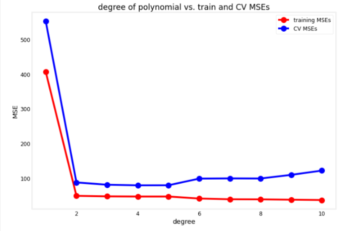
Choosing Model
We want to choose one that perrforms well both on the training and cross validatioin set, this means it was able to learn the patterns from the training set without overfitting.
# Get the model with the lowest CV MSE (add 1 because list indices start at 0)
# This also corresponds to the degree of the polynomial added
degree = np.argmin(cv_mses) + 1
print(f"Lowest CV MSE is found in the model with degree={degree}")
# Add polynomial features to the test set
X_test_mapped = polys[degree-1].transform(x_test)

# Scale the test set
X_test_mapped_scaled = scalers[degree-1].transform(X_test_mapped)

# Compute the test MSE
yhat = models[degree-1].predict(X_test_mapped_scaled)
test_mse = mean_squared_error(y_test, yhat) / 2

print(f"Training MSE: {train_mses[degree-1]:.2f}")
print(f"Cross Validation MSE: {cv_mses[degree-1]:.2f}")
print(f"Test MSE: {test_mse:.2f}")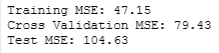
Neural Networks
Prepare Data
The default degree is set to 1 to indicate that it will just use x_train, x_cv, and x_test as is (i.e. without any additional polynomial features).
# Add polynomial features
degree = 1
poly = PolynomialFeatures(degree, include_bias=False)
X_train_mapped = poly.fit_transform(x_train)
X_cv_mapped = poly.transform(x_cv)
X_test_mapped = poly.transform(x_test)
Scale Features
# Scale the features using the z-score
scaler = StandardScaler()
X_train_mapped_scaled = scaler.fit_transform(X_train_mapped)
X_cv_mapped_scaled = scaler.transform(X_cv_mapped)
X_test_mapped_scaled = scaler.transform(X_test_mapped)
Build & Train
# Initialize lists that will contain the errors for each model
nn_train_mses = []
nn_cv_mses = []
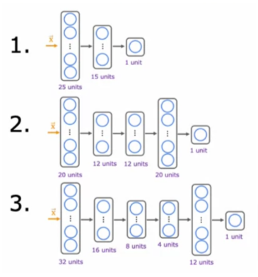
# Build the models
nn_models = utils.build_models()
# Loop over the the models
for model in nn_models:
# Setup the loss and optimizer
model.compile(
loss='mse',
optimizer=tf.keras.optimizers.Adam(learning_rate=0.1),
)
print(f"Training {model.name}...")
# Train the model
model.fit(
X_train_mapped_scaled, y_train,
epochs=300,
verbose=0
)
print("Done!\n")
# Record the training MSEs
yhat = model.predict(X_train_mapped_scaled)
train_mse = mean_squared_error(y_train, yhat) / 2
nn_train_mses.append(train_mse)
# Record the cross validation MSEs
yhat = model.predict(X_cv_mapped_scaled)
cv_mse = mean_squared_error(y_cv, yhat) / 2
nn_cv_mses.append(cv_mse)
# print results
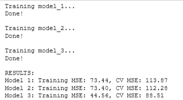
print("RESULTS:")
for model_num in range(len(nn_train_mses)):
print(
f"Model {model_num+1}: Training MSE: {nn_train_mses[model_num]:.2f}, " +
f"CV MSE: {nn_cv_mses[model_num]:.2f}"
)
Select Model
From the recorded errors, you can decide which is the best model for your application. Look at the results above and see if you agree with the selected model_num below. Finally, you will compute the test error to estimate how well it generalizes to new examples.
# Select the model with the lowest CV MSE
model_num = 3

# Compute the test MSE
yhat = nn_models[model_num-1].predict(X_test_mapped_scaled)
test_mse = mean_squared_error(y_test, yhat) / 2

print(f"Selected Model: {model_num}")
print(f"Training MSE: {nn_train_mses[model_num-1]:.2f}")
print(f"Cross Validation MSE: {nn_cv_mses[model_num-1]:.2f}")
print(f"Test MSE: {test_mse:.2f}")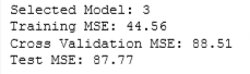
Classification Model
# Load the dataset from a text file
data = np.loadtxt('./data/data_w3_ex2.csv', delimiter=',')

# Split the inputs and outputs into separate arrays
x_bc = data[:,:-1]
y_bc = data[:,-1]

# Convert y into 2-D because the commands later will require it (x is already 2-D)
y_bc = np.expand_dims(y_bc, axis=1)

print(f"the shape of the inputs x is: {x_bc.shape}")
print(f"the shape of the targets y is: {y_bc.shape}")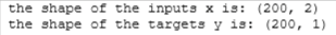
utils.plot_bc_dataset(x=x_bc, y=y_bc, title="x1 vs. x2")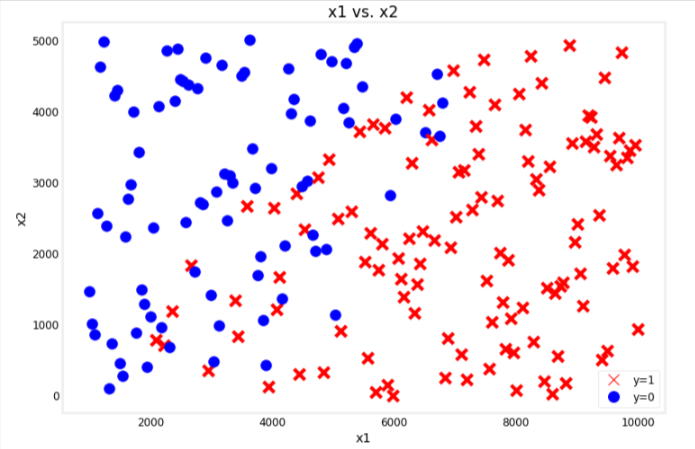
Split Dataset
from sklearn.model_selection import train_test_split

# Get 60% of the dataset as the training set. Put the remaining 40% in temporary variables.
x_bc_train, x_, y_bc_train, y_ = train_test_split(x_bc, y_bc, test_size=0.40, random_state=1)

# Split the 40% subset above into two: one half for cross validation and the other for the test set
x_bc_cv, x_bc_test, y_bc_cv, y_bc_test = train_test_split(x_, y_, test_size=0.50, random_state=1)

# Delete temporary variables
del x_, y_

print(f"the shape of the training set (input) is: {x_bc_train.shape}")
print(f"the shape of the training set (target) is: {y_bc_train.shape}\n")
print(f"the shape of the cross validation set (input) is: {x_bc_cv.shape}")
print(f"the shape of the cross validation set (target) is: {y_bc_cv.shape}\n")
print(f"the shape of the test set (input) is: {x_bc_test.shape}")
print(f"the shape of the test set (target) is: {y_bc_test.shape}")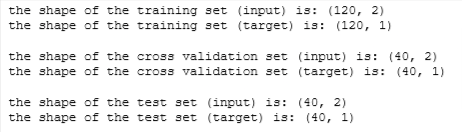
# Scale the features

# Initialize the class
scaler_linear = StandardScaler()

# Compute the mean and standard deviation of the training set then transform it
x_bc_train_scaled = scaler_linear.fit_transform(x_bc_train)
x_bc_cv_scaled = scaler_linear.transform(x_bc_cv)
x_bc_test_scaled = scaler_linear.transform(x_bc_test)
Evaluate Error
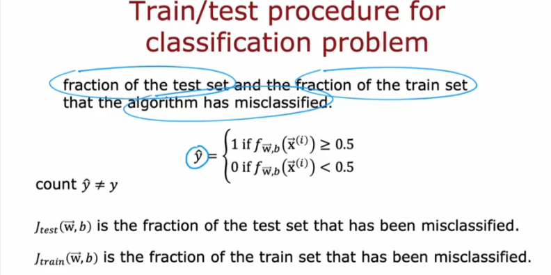
For classification, you can get a similar metric by getting the fraction of the data that the model has misclassified. For example, if your model made wrong predictions for 2 samples out of 5, then you will report an error of 40% or 0.4. The code below demonstrates this using a for-loop and also with Numpy’s mean() function.
# Sample model output
probabilities = np.array([0.2, 0.6, 0.7, 0.3, 0.8])

# Apply a threshold to the model output. If greater than 0.5, set to 1. Else 0.
predictions = np.where(probabilities >= 0.5, 1, 0)

# Ground truth labels
ground_truth = np.array([1, 1, 1, 1, 1])

# Initialize counter for misclassified data
misclassified = 0

# Get number of predictions
num_predictions = len(predictions)

# Loop over each prediction
for i in range(num_predictions):

    # Check if it matches the ground truth
    if predictions[i] != ground_truth[i]:

        # Add one to the counter if the prediction is wrong
        misclassified += 1

# Compute the fraction of the data that the model misclassified
fraction_error = misclassified/num_predictions

print(f"probabilities: {probabilities}")
print(f"predictions with threshold=0.5: {predictions}")
print(f"targets: {ground_truth}")
print(f"fraction of misclassified data (for-loop): {fraction_error}")
print(f"fraction of misclassified data (with np.mean()): {np.mean(predictions != ground_truth)}")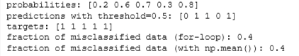
Build & Train
# Initialize lists that will contain the errors for each model
nn_train_error = []
nn_cv_error = []

# Build the models
models_bc = utils.build_models()

# Loop over each model
for model in models_bc:

    # Setup the loss and optimizer
    model.compile(
    loss=tf.keras.losses.BinaryCrossentropy(from_logits=True),
    optimizer=tf.keras.optimizers.Adam(learning_rate=0.01),
    )

    print(f"Training {model.name}...")

    # Train the model
    model.fit(
        x_bc_train_scaled, y_bc_train,
        epochs=200,
        verbose=0
    )

    print("Done!\n")

    # Set the threshold for classification
    threshold = 0.5

    # Record the fraction of misclassified examples for the training set
    yhat = model.predict(x_bc_train_scaled)
    yhat = tf.math.sigmoid(yhat)
    yhat = np.where(yhat >= threshold, 1, 0)
    train_error = np.mean(yhat != y_bc_train)
    nn_train_error.append(train_error)

    # Record the fraction of misclassified examples for the cross validation set
    yhat = model.predict(x_bc_cv_scaled)
    yhat = tf.math.sigmoid(yhat)
    yhat = np.where(yhat >= threshold, 1, 0)
    cv_error = np.mean(yhat != y_bc_cv)
    nn_cv_error.append(cv_error)

# Print the result
for model_num in range(len(nn_train_error)):
    print(
        f"Model {model_num+1}: Training Set Classification Error: {nn_train_error[model_num]:.5f}, " +
        f"CV Set Classification Error: {nn_cv_error[model_num]:.5f}"
        )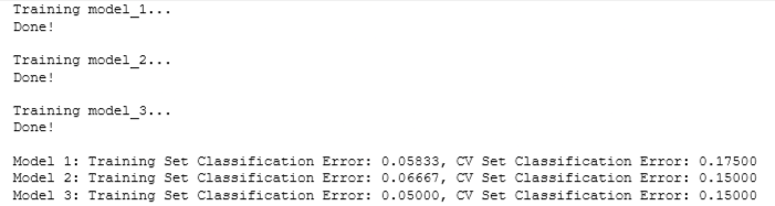
From the output above, you can choose which one performed best. If there is a tie on the cross validation set error, then you can add another criteria to break it. For example, you can choose the one with a lower training error. A more common approach is to choose the smaller model because it saves computational resources. In our example, Model 1 is the smallest and Model 3 is the largest.
Finally, you can compute the test error to report the model’s generalization error.
# Select the model with the lowest error
model_num = 3

# Compute the test error
yhat = models_bc[model_num-1].predict(x_bc_test_scaled)
yhat = tf.math.sigmoid(yhat)
yhat = np.where(yhat >= threshold, 1, 0)
nn_test_error = np.mean(yhat != y_bc_test)

print(f"Selected Model: {model_num}")
print(f"Training Set Classification Error: {nn_train_error[model_num-1]:.4f}")
print(f"CV Set Classification Error: {nn_cv_error[model_num-1]:.4f}")
print(f"Test Set Classification Error: {nn_test_error:.4f}")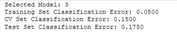
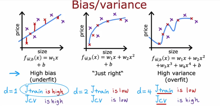
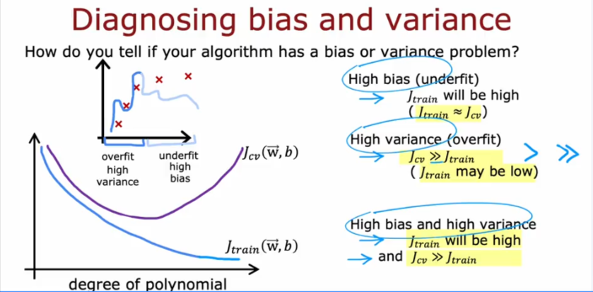
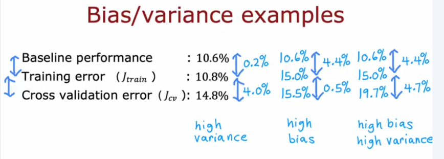
Bias & Variance
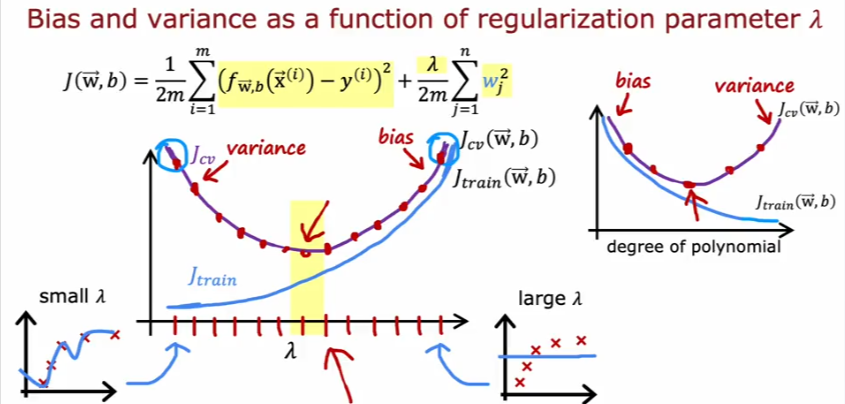
Regularization
Baseline Performance
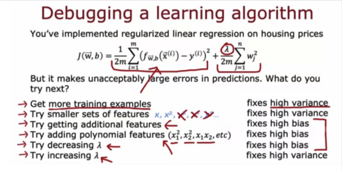
Debugging Algorithm