import numpy as np
import tensorflow as tf
from tensorflow.keras.models import Sequential
from tensorflow.keras.layers import Dense
from tensorflow.keras.activations import linear, relu, sigmoid
%matplotlib widget
import matplotlib.pyplot as plt
plt.style.use('./deeplearning.mplstyle')

import logging
logging.getLogger("tensorflow").setLevel(logging.ERROR)
tf.autograph.set_verbosity(0)

from public_tests import *

from autils import *
from lab_utils_softmax import plt_softmax
np.set_printoptions(precision=2)NN in Numpy - Digit Recognition III
This is a continuation of Digit Recog I & II but we will use the more precise and more efficient method to classify the data:
We will use a neural network to recognize ten handwritten digits, 0-9. This is a multiclass classification task where one of n choices is selected. Automated handwritten digit recognition is widely used today - from recognizing zip codes (postal codes) on mail envelopes to recognizing amounts written on bank checks.
Libraries
.
Plot
We’ve seen this before, but let’s plot it out as a reminder:
plt_act_trio()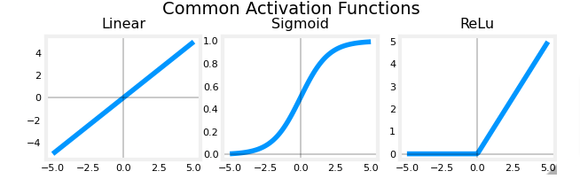
Recap
ReLU
Here is a familiar image we used earlier
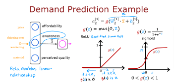
The example from the previous pages shown above shows an application of the ReLU. In this example, the derived “awareness” feature is not binary but has a continuous range of values. The sigmoid is best for on/off or binary situations. The ReLU provides a continuous linear relationship. Additionally it has an ‘off’ range where the output is zero. The “off” feature makes the ReLU a Non-Linear activation. Why is this needed? This enables multiple units to contribute to to the resulting function without interfering.
Softmax
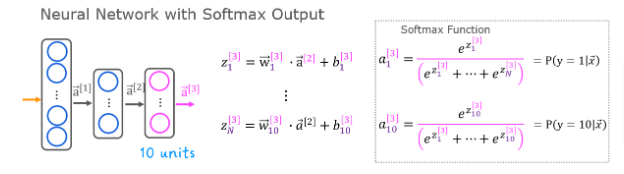
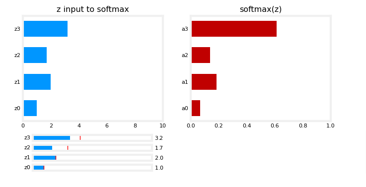
A multiclass neural network generates N outputs. One output is selected as the predicted answer. In the output layer, a vector 𝐳z is generated by a linear function which is fed into a softmax function. The softmax function converts 𝐳z into a probability distribution as described below. After applying softmax, each output will be between 0 and 1 and the outputs will sum to 1. They can be interpreted as probabilities. The larger inputs to the softmax will correspond to larger output probabilities.
The softmax function can be written as
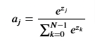
where z=w.x + b and N is the number of feature/categories in the output layer
Numpy Softmax
def my_softmax(z):
    """ Softmax converts a vector of values to a probability distribution.
    Args:
      z (ndarray (N,))  : input data, N features
    Returns:
      a (ndarray (N,))  : softmax of z
    """
    z = np.exp(z)
    a = z/np.sum(z)
    return a
View
Using a function in the library we test our function compared to the one TF utilizes:
z = np.array([1., 2., 3., 4.])
a = my_softmax(z)
atf = tf.nn.softmax(z)
print(f"my_softmax(z):         {a}")
print(f"tensorflow softmax(z): {atf}")

test_my_softmax(my_softmax)
Note that as we vary the value of z inputs, the exponential in the numerator magnifies small differences in the values. Also note that the output values always add up to 1
So now let’s use NN to recognize ten handwritten digits 0-9
Project
Load Data
We will start by loading the dataset for this task.
- The
load_data()function shown below loads the data into variablesXandy
The data set contains 5000 training examples of handwritten digits 11.
Each training example is a 20-pixel x 20-pixel grayscale image of the digit.
Each pixel is represented by a floating-point number indicating the grayscale intensity at that location.
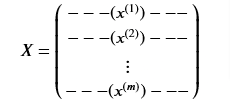
The 20 by 20 grid of pixels is “unrolled” into a 400-dimensional vector.
Each training examples becomes a single row in our data matrix
X.This gives us a 5000 x 400 matrix
Xwhere every row is a training example of a handwritten digit image.
The second part of the training set is a 5000 x 1 dimensional vector
ythat contains labels for the training sety = 0if the image is of the digit0,y = 4if the image is of the digit4and so on.
# load dataset
X, y = load_data()
print ('The first element of X is: ', X[0])
print ('The first element of y is: ', y[0,0])
print ('The last element of y is: ', y[-1,0])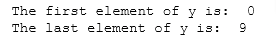
print ('The shape of X is: ' + str(X.shape))
print ('The shape of y is: ' + str(y.shape))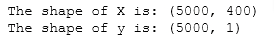
Visualize Data
We will begin by visualizing a subset of the training set.
- In the cell below, the code randomly selects 64 rows from
X, maps each row back to a 20 pixel by 20 pixel grayscale image and displays the images together. - The label for each image is displayed above the image
import warnings
warnings.simplefilter(action='ignore', category=FutureWarning)
# You do not need to modify anything in this cell

m, n = X.shape

fig, axes = plt.subplots(8,8, figsize=(5,5))
fig.tight_layout(pad=0.13,rect=[0, 0.03, 1, 0.91]) #[left, bottom, right, top]

#fig.tight_layout(pad=0.5)
widgvis(fig)
for i,ax in enumerate(axes.flat):
    # Select random indices
    random_index = np.random.randint(m)

    # Select rows corresponding to the random indices and
    # reshape the image
    X_random_reshaped = X[random_index].reshape((20,20)).T

    # Display the image
    ax.imshow(X_random_reshaped, cmap='gray')

    # Display the label above the image
    ax.set_title(y[random_index,0])
    ax.set_axis_off()
    fig.suptitle("Label, image", fontsize=14)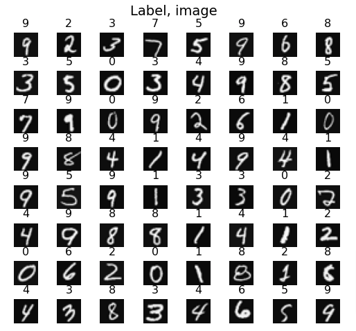
Layout Model
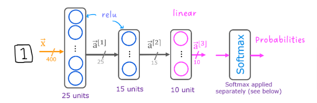
The neural network we will use is shown in the figure below.
This has two dense layers with ReLU activations followed by an output layer with a linear activation.
Recall that our inputs are pixel values of digit images.
Since the images are of size 20×2020×20, this gives us 400400 inputs
The parameters have dimensions that are sized for a neural network with 2525 units in layer 1, 1515 units in layer 2 and 1010 output units in layer 3, one for each digit.
Recall that the dimensions of these parameters is determined as follows:
If network has 𝑠𝑖𝑛sin units in a layer and 𝑠𝑜𝑢𝑡sout units in the next layer, then
𝑊W will be of dimension 𝑠𝑖𝑛×𝑠𝑜𝑢𝑡sin×sout.
𝑏b will be a vector with 𝑠𝑜𝑢𝑡sout elements
Therefore, the shapes of
W, andb, arelayer1: The shape of
W1is (400, 25) and the shape ofb1is (25,)layer2: The shape of
W2is (25, 15) and the shape ofb2is: (15,)
The bias vector
bcould be represented as a 1-D (n,) or 2-D (n,1) array. Tensorflow utilizes a 1-D representation and this lab will maintain that convention:
TF Implementation
ReLU
As described in the pages before, numerical stability is improved if the softmax is grouped with the loss function rather than the output layer during training. This has implications when building the model and using the model.
Building:
- The final Dense layer should use a ‘linear’ activation. This is effectively no activation.
- The
model.compilestatement will indicate this by includingfrom_logits=True.loss=tf.keras.losses.SparseCategoricalCrossentropy(from_logits=True) - This does not impact the form of the target. In the case of SparseCategorialCrossentropy, the target is the expected digit, 0-9.
Using the model:
- The outputs are not probabilities. If output probabilities are desired, apply a softmax function.
tf.random.set_seed(1234) # for consistent results
model = Sequential(
    [
        tf.keras.Input(shape=(400,)),
        Dense(25, activation = 'relu', name = "L1"),
        Dense(15, activation = 'relu', name = "L2"),
        Dense(10 , activation = 'linear', name = "L3")
    ], name = "my_model"
)
model.summary()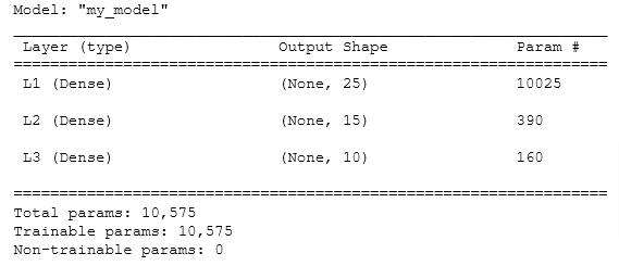
Layers & Weights
Let’s look at the weights to see if TF produced the same dimensions as we calculated above
[layer1, layer2, layer3] = model.layers#### Examine Weights shapes
W1,b1 = layer1.get_weights()
W2,b2 = layer2.get_weights()
W3,b3 = layer3.get_weights()
print(f"W1 shape = {W1.shape}, b1 shape = {b1.shape}")
print(f"W2 shape = {W2.shape}, b2 shape = {b2.shape}")
print(f"W3 shape = {W3.shape}, b3 shape = {b3.shape}")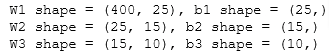
Loss
- define a loss function,
SparseCategoricalCrossentropyand indicates the softmax should be included with the loss calculation by addingfrom_logits=True) - defines an optimizer. A popular choice is Adaptive Moment (Adam) which was described in lecture.
- In the fit statement, the number of epochs is set to 40, so run the training data 40 times
- Since we have 5000 examples in our data, and TF has a default batch size of 32, it means that to process the 5000 examples we will need 157 batches.
- That’s what the output below displays, which batch is being processed…
model.compile(
    loss=tf.keras.losses.SparseCategoricalCrossentropy(from_logits=True),
    optimizer=tf.keras.optimizers.Adam(learning_rate=0.001),
)

history = model.fit(
    X,y,
    epochs=40
)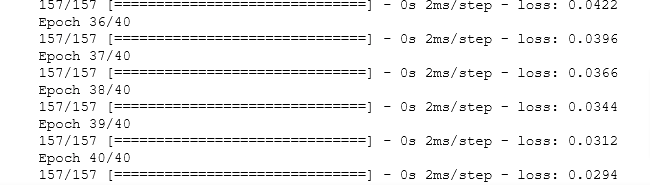
As you see above the loss decreases (hopefully) as the number of iterations increases. This we learned in GD earlier, by monitoring the cost. Ideally, the cost will decrease as the number of iterations of the algorithm increases. Tensorflow refers to the cost as loss. Above, you saw the loss displayed each epoch as model.fit was executing. The .fit method returns a variety of metrics including the loss. This is captured in the history variable above. This can be used to examine the loss in a plot as shown below
plot_loss_tf(history)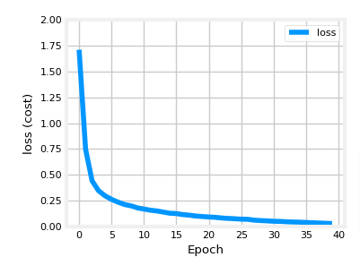
Predit
Index Output
Use Keras predict(). The image we will use X[1015] contains an image of a 2
image_of_two = X[1015]
display_digit(image_of_two)

prediction = model.predict(image_of_two.reshape(1,400))  # prediction

print(f" predicting a Two: \n{prediction}")
print(f" Largest Prediction index: {np.argmax(prediction)}")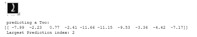
you can see the largest prediction[2] is the third element which is the number 2. If the output requires a probability, then softmax is required
Predict Probability
Remember we covered this in the optimization page, now we have to convert it using
prediction_p = tf.nn.softmax(prediction)

print(f" predicting a Two. Probability vector: \n{prediction_p}")
print(f"Total of predictions: {np.sum(prediction_p):0.3f}")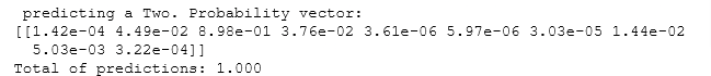
Predict a Digit
So now we want to extract the index of the largest probability yielded above, this is done with argmax()
yhat = np.argmax(prediction_p)

print(f"np.argmax(prediction_p): {yhat}")
Predict vs Actual
Let’s compare the predicted values against the true labels for a random sample of 64 digits.
import warnings
warnings.simplefilter(action='ignore', category=FutureWarning)
# You do not need to modify anything in this cell
m, n = X.shape
fig, axes = plt.subplots(8,8, figsize=(5,5))
fig.tight_layout(pad=0.13,rect=[0, 0.03, 1, 0.91]) #[left, bottom, right, top]
widgvis(fig)
for i,ax in enumerate(axes.flat):
# Select random indices
random_index = np.random.randint(m)
# Select rows corresponding to the random indices and
# reshape the image
X_random_reshaped = X[random_index].reshape((20,20)).T
# Display the image
ax.imshow(X_random_reshaped, cmap='gray')
# Predict using the Neural Network
prediction = model.predict(X[random_index].reshape(1,400))
prediction_p = tf.nn.softmax(prediction)
yhat = np.argmax(prediction_p)
# Display the label above the image
ax.set_title(f"{y[random_index,0]},{yhat}",fontsize=10)
ax.set_axis_off()
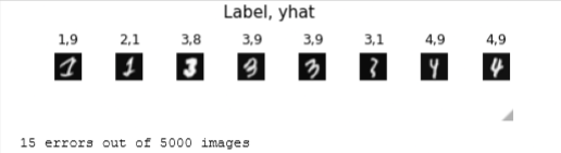
fig.suptitle("Label, yhat", fontsize=14)
plt.show()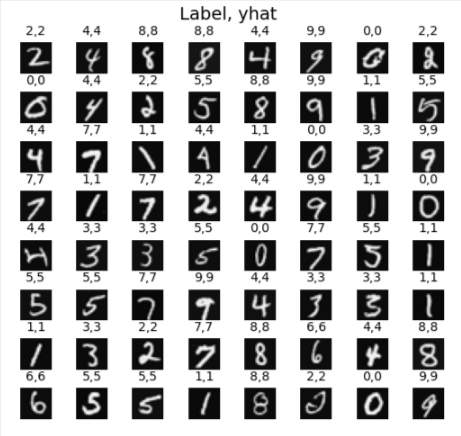
Errors
If we increase the number of epochs, we can eliminate more errors.
print( f"{display_errors(model,X,y)} errors out of {len(X)} images")