import numpy as np
import matplotlib.pyplot as plt
from lab_utils_multi import zscore_normalize_features, run_gradient_descent_feng
np.set_printoptions(precision=2) # reduced display precision on numpy arraysPolynomial Regression
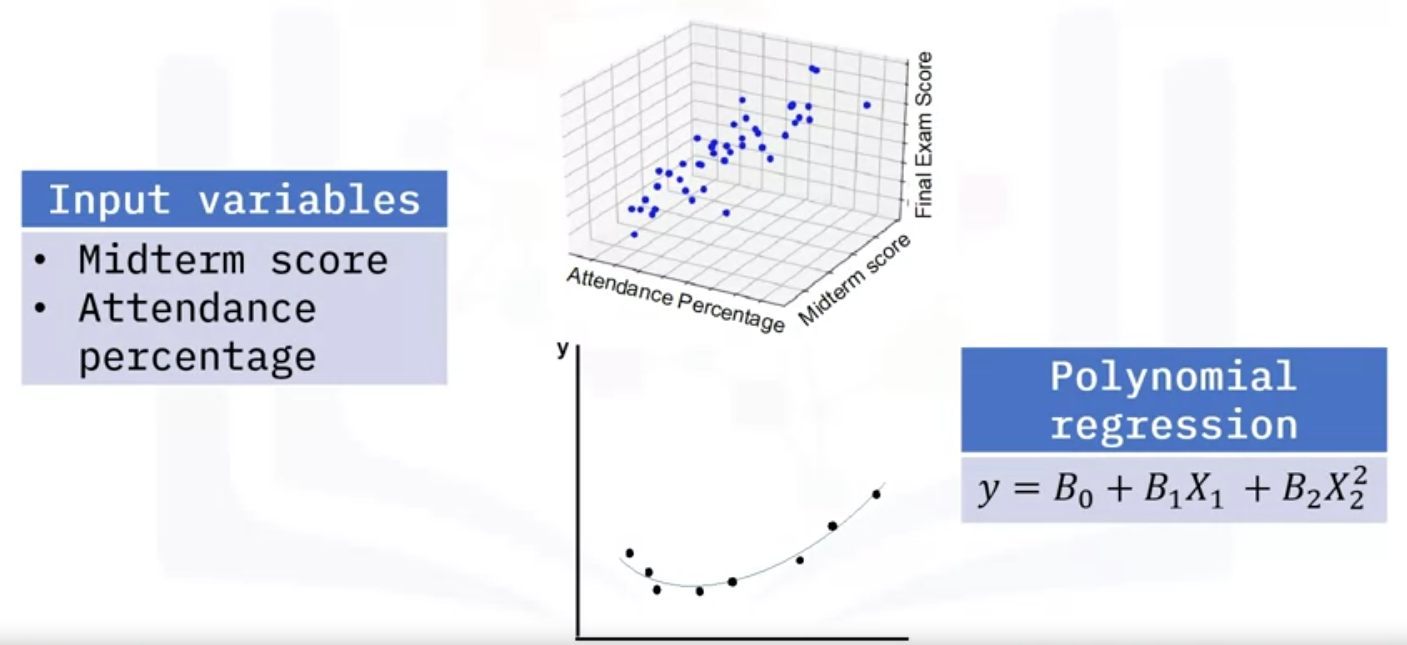
In the final exam problem, you can have more variables that predict the outcome of the final exam score.
- You may have two variables instead, such as midterm score and attendance percentage.
- In this case, you would be dealing with a 3D graph with two slopes:
- one for the relationship between midterm score and final score,
- and one for attendance percentage and final score.
- imagine you have 10 variables.
- This model uses a polynomial of degree two to account for the nonlinear relationship.
Now that we know that we can engineer some of our features we can also fit curves to our data instead of linear (straight lines). Above we were considering a scenario where the data was non-linear. Let’s try using what we know so far to fit a non-linear curve. We’ll start with a simple quadratic: y = 1 + x2
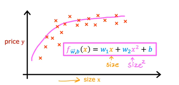
- So going back to our housing data from the previous linear regression model, and let’s say our data looks like the plot below
- We can try to fit a curve to the data using the square of the size feature and add it to the linear regression formula we used before as shown in the image below
- Then you realize that the quadratic function eventually comes down and we know our data/price values don’t come down
- So then we can add an x (size feature) cubed to the function or even to more powers to fit the data better
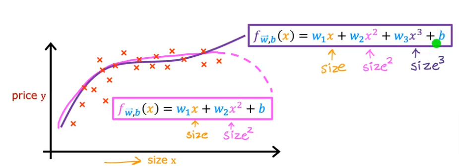
- In this case feature scaling becomes extremely important because as you raise a feature to a third power
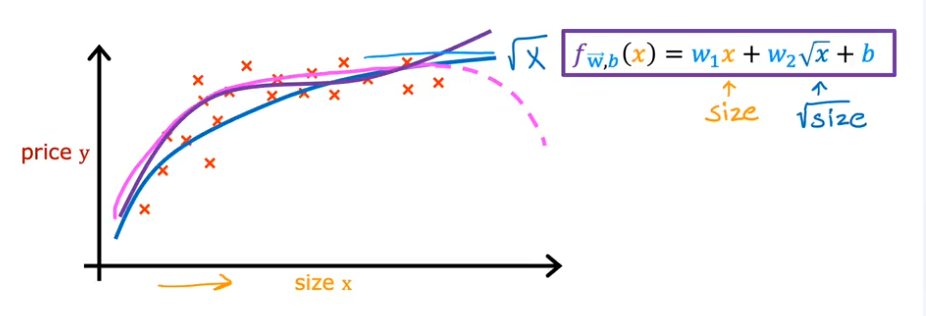
- Another option to use instead of square, cube…. is to use square root, because we know the square root curve continuously increases at a small rate and the feature scaling doesn’t become so magnified
- So what feature do we use? and which model? We’ll cover soon
- Scikit can be used to access many of these functions as a package
Code
What if your features/data are non-linear or are combinations of features? For example, Housing prices do not tend to be linear with living area but penalize very small or very large houses resulting in the curves shown in the graphic above. How can we use the machinery of linear regression to fit this curve? Recall, the ‘machinery’ we have is the ability to modify the parameters w, b in (1) to ‘fit’ the equation to the training data. However, no amount of adjusting of w,b in (1) will achieve a fit to a non-linear curve.
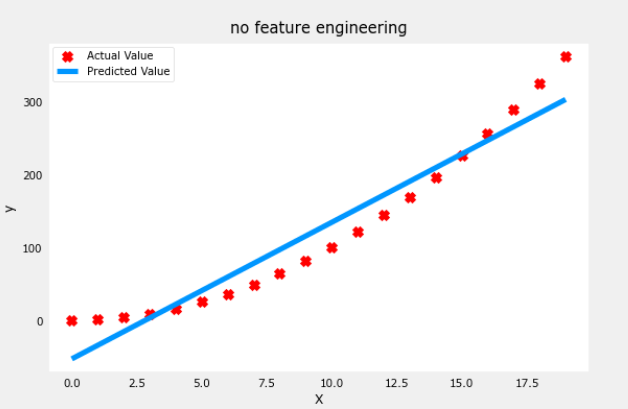
Let’s start with a simple y = 1+x2 quadratic formula and as you see below it is not a great fit
- note the values of w and b
# create target data
x = np.arange(0, 20, 1)
y = 1 + x**2
X = x.reshape(-1, 1)

model_w,model_b = run_gradient_descent_feng(X,y,iterations=1000, alpha = 1e-2)

plt.scatter(x, y, marker='x', c='r', label="Actual Value"); plt.title("no feature engineering")
plt.plot(x,X@model_w + model_b, label="Predicted Value");  plt.xlabel("X"); plt.ylabel("y"); plt.legend(); plt.show()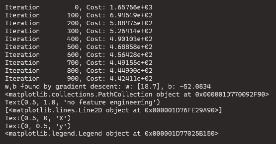
Feature Engineering
Let’s try feature engineering by taking x and replacing with x2
- Notice the values of w and b printed right above the graph:
w,b found by gradient descent: w: [1.], b: 0.0490. - Gradient descent modified our initial values of w,b to be (1.0,0.049) or a model of y=1∗x02+0.049, very close to our target of y=1∗x02+1. If you ran it longer, it could be a better match.
# create target data
x = np.arange(0, 20, 1)
y = 1 + x**2

# Engineer features
X = x**2      #<-- added engineered feature
X = X.reshape(-1, 1) #X should be a 2-D Matrix
model_w,model_b = run_gradient_descent_feng(X, y, iterations=10000, alpha = 1e-5)
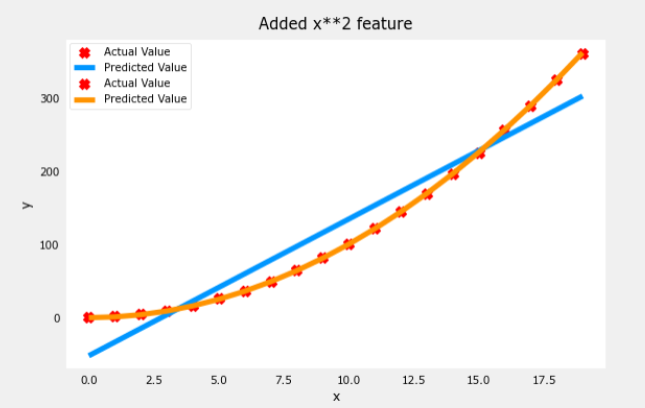
plt.scatter(x, y, marker='x', c='r', label="Actual Value"); plt.title("Added x**2 feature")
plt.plot(x, np.dot(X,model_w) + model_b, label="Predicted Value"); plt.xlabel("x"); plt.ylabel("y"); plt.legend(); plt.show()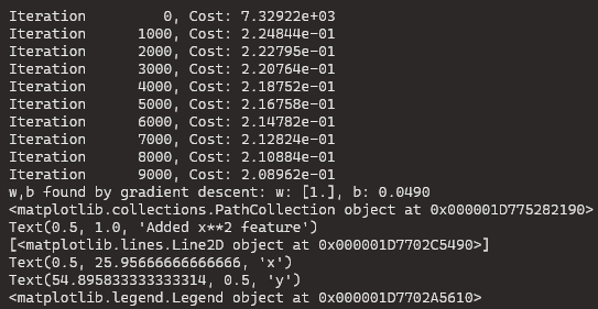
How many Features
So how do we know how many features to use or which are required? One can add a variety of potential features to try and find the most useful ones. Let’s try

# create target data
x = np.arange(0, 20, 1)
y = x**2

# engineer features .
X = np.c_[x, x**2, x**3]   #<-- added engineered feature
model_w,model_b = run_gradient_descent_feng(X, y, iterations=10000, alpha=1e-7)
plt.scatter(x, y, marker='x', c='r', label="Actual Value"); plt.title("x, x**2, x**3 features")
plt.plot(x, X@model_w + model_b, label="Predicted Value"); plt.xlabel("x"); plt.ylabel("y"); plt.legend(); plt.show()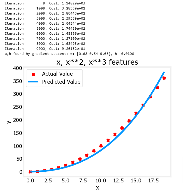
Note the value of w (an array now) and b which means that after training the model looks like this:
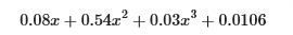
Gradient descent has emphasized the data that is the best fit to the x2 data by increasing the w1 term relative to the others. If you were to run for a very long time, it would continue to reduce the impact of the other terms.
Gradient descent is picking the ‘correct’ features for us by emphasizing its associated parameter
Let’s review this idea:
- Intially, the features were re-scaled so they are comparable to each other
- less weight value implies less important/correct feature, and in extreme, when the weight becomes zero or very close to zero, the associated feature useful in fitting the model to the data.
- above, after fitting, the weight associated with the x2 feature is much larger than the weights for x or x3 as it is the most useful in fitting the data.
Which Feature
Above, polynomial features were chosen based on how well they matched the target data. Another way to think about this is to note that we are still using linear regression once we have created new features. Given that, the best features will be linear relative to the target. This is best understood with an example.
Let’s see how each feature influences the curve.
- You can easily see below that the x2 feature mapped against the target value y is linear.
# create target data
x = np.arange(0, 20, 1)
y = x**2

# engineer features .
X = np.c_[x, x**2, x**3]   #<-- added engineered feature
X_features = ['x','x^2','x^3']fig,ax=plt.subplots(1, 3, figsize=(12, 3), sharey=True)
for i in range(len(ax)):
ax[i].scatter(X[:,i],y)
ax[i].set_xlabel(X_features[i])
ax[0].set_ylabel("y")
plt.show()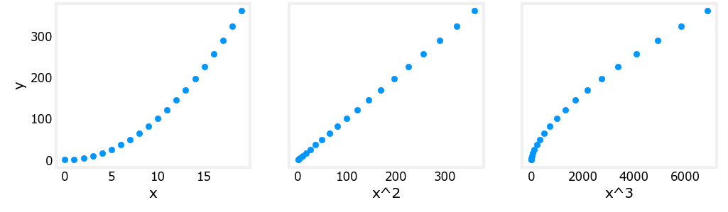
Scaling Z-Score Normalization
As we learned in a previous page, if the data set has features with significantly different scales, one should apply feature scaling to speed gradient descent. Since we have x to 3 different power in the formula, let’s apply Z-score normalization to our example.
Normalize First
# create target data
x = np.arange(0,20,1)
X = np.c_[x, x**2, x**3]
print(f"Peak to Peak range by column in Raw        X:{np.ptp(X,axis=0)}")

# add mean_normalization
X = zscore_normalize_features(X)
print(f"Peak to Peak range by column in Normalized X:{np.ptp(X,axis=0)}")
Run The Model
Let’s try with a more aggressive value of alpha
x = np.arange(0,20,1)
y = x**2

X = np.c_[x, x**2, x**3]
X = zscore_normalize_features(X)

model_w, model_b = run_gradient_descent_feng(X, y, iterations=100000, alpha=1e-1)

plt.scatter(x, y, marker='x', c='r', label="Actual Value"); plt.title("Normalized x x**2, x**3 feature")
plt.plot(x,X@model_w + model_b, label="Predicted Value"); plt.xlabel("x"); plt.ylabel("y"); plt.legend(); plt.show()
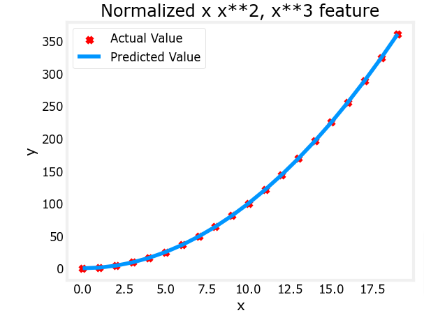
Feature scaling allows this to converge much faster.
Note again the values of w. The w1 term, which is the x2 term is the most emphasized. Gradient descent has all but eliminated the x3 term.
Complex Engineering
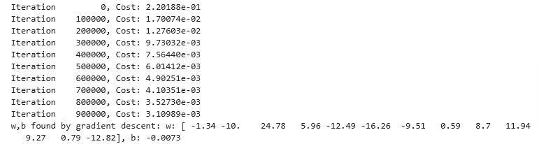
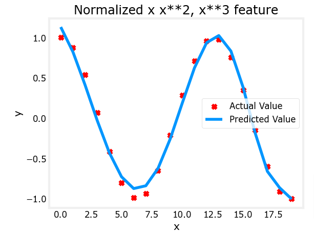
With feature engineering, even quite complex functions can be modeled
x = np.arange(0,20,1)
y = np.cos(x/2)

X = np.c_[x, x**2, x**3,x**4, x**5, x**6, x**7, x**8, x**9, x**10, x**11, x**12, x**13]
X = zscore_normalize_features(X)

model_w,model_b = run_gradient_descent_feng(X, y, iterations=1000000, alpha = 1e-1)

plt.scatter(x, y, marker='x', c='r', label="Actual Value"); plt.title("Normalized x x**2, x**3 feature")
plt.plot(x,X@model_w + model_b, label="Predicted Value"); plt.xlabel("x"); plt.ylabel("y"); plt.legend(); plt.show()