import numpy as np
import matplotlib.pyplot as plt
from lab_utils_multi import  load_house_data, run_gradient_descent
from lab_utils_multi import  norm_plot, plt_equal_scale, plot_cost_i_w
from lab_utils_common import dlc
np.set_printoptions(precision=2)
plt.style.use('./deeplearning.mplstyle')Learning Rate
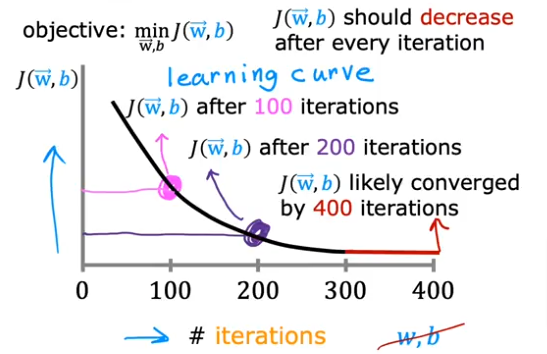
So now that we have scaled the features, and ready to train our model, how do we know that our Gradient Descent is actually converging and has reached the minimum cost value?
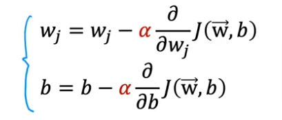
Here is the gradient descent formulas again with the learning rate in red with J(w,b) being the cost
What we have to remember that with the number of iterations we should expect the cost to get closer to zero or that the curve is no longer decreasing (slope change is closer to 0). The number of iterations could vary from 100 to thousands.
Plot
If we plot the learning curve with # of iterations and Cost value as the axes we get
Convergence Test
- Another way to check to see if our gradient descent is converging, would be using an automatic convergence test.
- We can set a value to be 10-3 = 0.001
- If our cost function decreases by <= .001 in an iteration, then we can declare convergence (means we found parameters w,b to get us a value close to global minimum)
- What’s hard is trying to figure out what that value should be
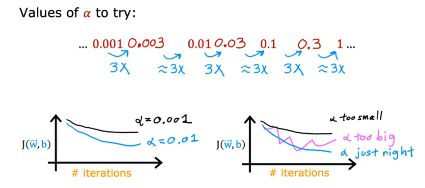
As we recall, if the learning rate is too large the gd might never converge, if too small it might take too long. So it would be advisable to try different values and plot them like this:
- Start out with a \({\alpha}\) = 0.001 and plot the results
- Then multiply it by 3 and try 0.003 and on an on till you see the learning rate closer to zero and has flattened out
Code
Setup
.
Load Data
# load the dataset
X_train, y_train = load_house_data()
X_features = ['size(sqft)','bedrooms','floors','age']
\({\alpha}\) = 9.9e-7
#set alpha to 9.9e-7
_, _, hist = run_gradient_descent(X_train, y_train, 10, alpha = 9.9e-7)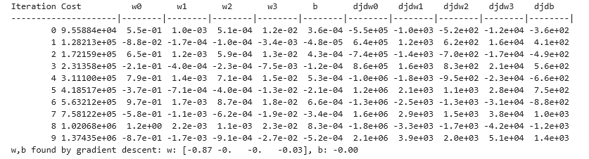
It appears the learning rate is too high. As you see the cost is increasing rather than decreasing, let’s see the plot of it:
The plot on the right shows the value of one of the parameters, w0. At each iteration, it is overshooting the optimal value and as a result, cost ends up increasing rather than approaching the minimum. Note that this is not a completely accurate picture as there are 4 parameters being modified each pass rather than just one. This plot is only showing w0 with the other parameters fixed at benign values. In this and later plots you may notice the blue and orange lines being slightly off.
plot_cost_i_w(X_train, y_train, hist)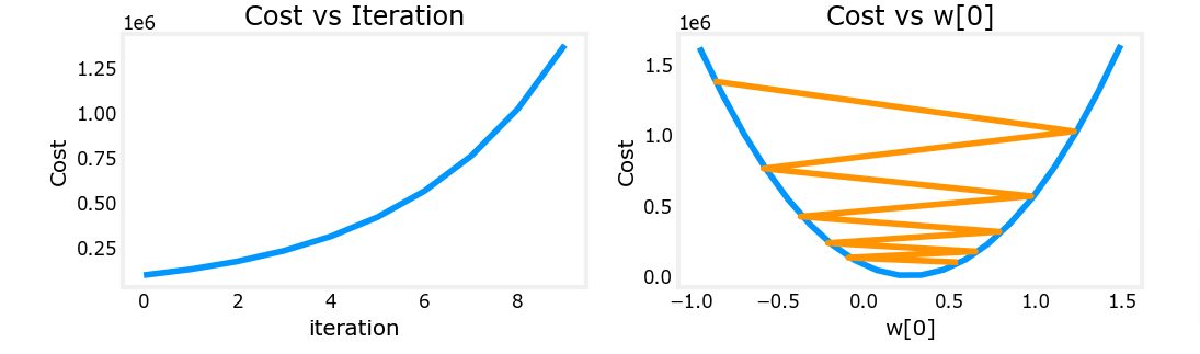
\({\alpha}\) = 9e-7
- Let’s try a smaller value
#set alpha to 9e-7
_,_,hist = run_gradient_descent(X_train, y_train, 10, alpha = 9e-7)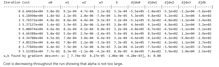
plot_cost_i_w(X_train, y_train, hist)
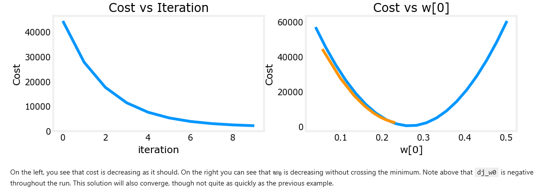
On the left, you see that cost is decreasing as it should. On the right, you can see that w0 is still oscillating around the minimum, but it is decreasing each iteration rather than increasing. Note above that dj_dw[0] changes sign with each iteration as w[0] jumps over the optimal value. This alpha value will converge. You can vary the number of iterations to see how it behaves.
\({\alpha}\) = 1e-7
- Let’s try yet another smaller value
#set alpha to 1e-7
_,_,hist = run_gradient_descent(X_train, y_train, 10, alpha = 1e-7)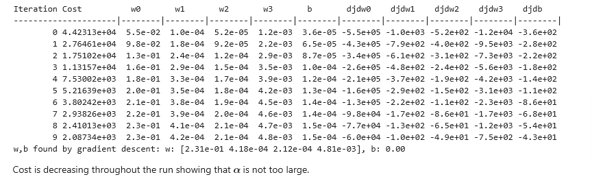
plot_cost_i_w(X_train,y_train,hist)