import copy, math
import numpy as np
%matplotlib widget
import matplotlib.pyplot as plt
from lab_utils_common import  dlc, plot_data, plt_tumor_data, sigmoid, compute_cost_logistic
from plt_quad_logistic import plt_quad_logistic, plt_prob
plt.style.use('./deeplearning.mplstyle')Gradient Descent
So how do we find the values for w and b to minimize the cost for the model?
Recall from previous work that we have to iterate over the entire training set and repeat while updating w & b simulteanously
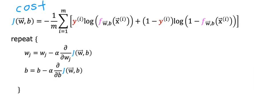
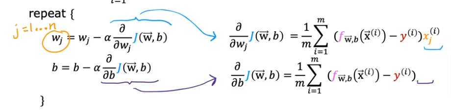
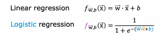
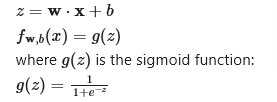
summarized as the same formula we used for linear regression
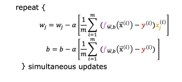
Yes except that for a logistic regression
Code
X_train = np.array([[0.5, 1.5], [1,1], [1.5, 0.5], [3, 0.5], [2, 2], [1, 2.5]])
y_train = np.array([0, 0, 0, 1, 1, 1])
fig,ax = plt.subplots(1,1,figsize=(4,4))
plot_data(X_train, y_train, ax)
ax.axis([0, 4, 0, 3.5])
ax.set_ylabel('$x_1$', fontsize=12)
ax.set_xlabel('$x_0$', fontsize=12)
plt.show()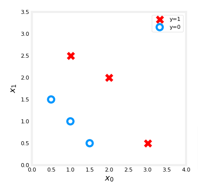
Gradient Descent
def compute_gradient_logistic(X, y, w, b):
    """
    Computes the gradient for logistic regression

    Args:
      X (ndarray (m,n): Data, m examples with n features
      y (ndarray (m,)): target values
      w (ndarray (n,)): model parameters
      b (scalar)      : model parameter
    Returns
      dj_dw (ndarray (n,)): The gradient of the cost w.r.t. the parameters w.
      dj_db (scalar)      : The gradient of the cost w.r.t. the parameter b.
    """
    m,n = X.shape
    dj_dw = np.zeros((n,))                           #(n,)
    dj_db = 0.

    for i in range(m):
        f_wb_i = sigmoid(np.dot(X[i],w) + b)          #(n,)(n,)=scalar
        err_i  = f_wb_i  - y[i]                       #scalar
        for j in range(n):
            dj_dw[j] = dj_dw[j] + err_i * X[i,j]      #scalar
        dj_db = dj_db + err_i
    dj_dw = dj_dw/m                                   #(n,)
    dj_db = dj_db/m                                   #scalar

    return dj_db, dj_dw
X_tmp = np.array([[0.5, 1.5], [1,1], [1.5, 0.5], [3, 0.5], [2, 2], [1, 2.5]])
y_tmp = np.array([0, 0, 0, 1, 1, 1])
w_tmp = np.array([2.,3.])
b_tmp = 1.
dj_db_tmp, dj_dw_tmp = compute_gradient_logistic(X_tmp, y_tmp, w_tmp, b_tmp)
print(f"dj_db: {dj_db_tmp}" )
print(f"dj_dw: {dj_dw_tmp.tolist()}" )Gradient Descent
def gradient_descent(X, y, w_in, b_in, alpha, num_iters):
    """
    Performs batch gradient descent

    Args:
      X (ndarray (m,n)   : Data, m examples with n features
      y (ndarray (m,))   : target values
      w_in (ndarray (n,)): Initial values of model parameters
      b_in (scalar)      : Initial values of model parameter
      alpha (float)      : Learning rate
      num_iters (scalar) : number of iterations to run gradient descent

    Returns:
      w (ndarray (n,))   : Updated values of parameters
      b (scalar)         : Updated value of parameter
    """
    # An array to store cost J and w's at each iteration primarily for graphing later
    J_history = []
    w = copy.deepcopy(w_in)  #avoid modifying global w within function
    b = b_in

    for i in range(num_iters):
        # Calculate the gradient and update the parameters
        dj_db, dj_dw = compute_gradient_logistic(X, y, w, b)

        # Update Parameters using w, b, alpha and gradient
        w = w - alpha * dj_dw
        b = b - alpha * dj_db

        # Save cost J at each iteration
        if i<100000:      # prevent resource exhaustion
            J_history.append( compute_cost_logistic(X, y, w, b) )

        # Print cost every at intervals 10 times or as many iterations if < 10
        if i% math.ceil(num_iters / 10) == 0:
            print(f"Iteration {i:4d}: Cost {J_history[-1]}   ")

    return w, b, J_history         #return final w,b and J history for graphing
Calculate GD
w_tmp  = np.zeros_like(X_train[0])
b_tmp  = 0.
alph = 0.1
iters = 10000

w_out, b_out, _ = gradient_descent(X_train, y_train, w_tmp, b_tmp, alph, iters)
print(f"\nupdated parameters: w:{w_out}, b:{b_out}")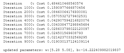
Plot
fig,ax = plt.subplots(1,1,figsize=(5,4))
# plot the probability
plt_prob(ax, w_out, b_out)

# Plot the original data
ax.set_ylabel(r'$x_1$')
ax.set_xlabel(r'$x_0$')
ax.axis([0, 4, 0, 3.5])
plot_data(X_train,y_train,ax)

# Plot the decision boundary
x0 = -b_out/w_out[0]
x1 = -b_out/w_out[1]
ax.plot([0,x0],[x1,0], c=dlc["dlblue"], lw=1)
plt.show()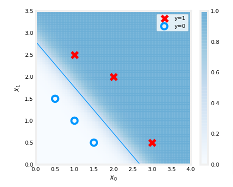
In the plot above:
- the shading reflects the probability y=1 (result prior to decision boundary)
- the decision boundary is the line at which the probability = 0.5
One Variable Dataset
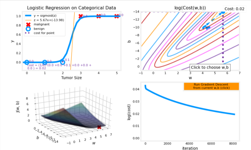
Let’s return to a one-variable data set. With just two parameters, 𝑤w, 𝑏b, it is possible to plot the cost function using a contour plot to get a better idea of what gradient descent is up to.
x_train = np.array([0., 1, 2, 3, 4, 5])
y_train = np.array([0,  0, 0, 1, 1, 1])
The data points with label 𝑦=1y=1 are shown as red crosses, while the data points with label 𝑦=0y=0 are shown as blue circles.
fig,ax = plt.subplots(1,1,figsize=(4,3))
plt_tumor_data(x_train, y_train, ax)
plt.show()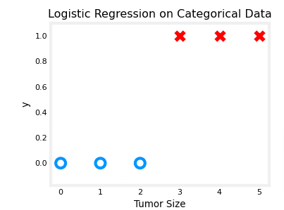
In the plot below, try:
- changing 𝑤w and 𝑏b by clicking within the contour plot on the upper right.
- changes may take a second or two
- note the changing value of cost on the upper left plot.
- note the cost is accumulated by a loss on each example (vertical dotted lines)
- run gradient descent by clicking the orange button.
note the steadily decreasing cost (contour and cost plot are in log(cost)
clicking in the contour plot will reset the model for a new run
- to reset the plot, rerun the cell
w_range = np.array([-1, 7])
b_range = np.array([1, -14])
quad = plt_quad_logistic( x_train, y_train, w_range, b_range )