import numpy as np
%matplotlib widget
import matplotlib.pyplot as plt
from plt_overfit import overfit_example, output
from lab_utils_common import sigmoid
np.set_printoptions(precision=8)Overfitting

Underfitting
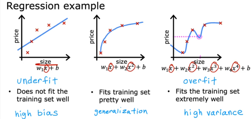
Before we get to overfitting we can actually cover Underfitting, or High Bias
Generalization
When it fits pretty well or generalizes pretty well on new data
Overfitting
Fits too perfectly, and error is zero and has High Variance or Overfit, and it does not generalize well for new data
Solutions
Collect more data
Select Features Exclude/Use
One disadvantage is you eliminate some relevant features
Regularization
Reduce the size of parameters wj
Regularization
You shrink the effect of all the features by reducing the size of w and not worry about b (you could but it doesn’t have much of an effect)
We can modify the cost function to apply regularization
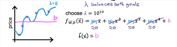
Let’s say we shrink the cost function to minimize wi for linear regression and we add large x values, so to minimize the effect of the new values is to lower w. When we eliminate the last two parts of the equation we are back to a fit that’s closer to the quadratic function
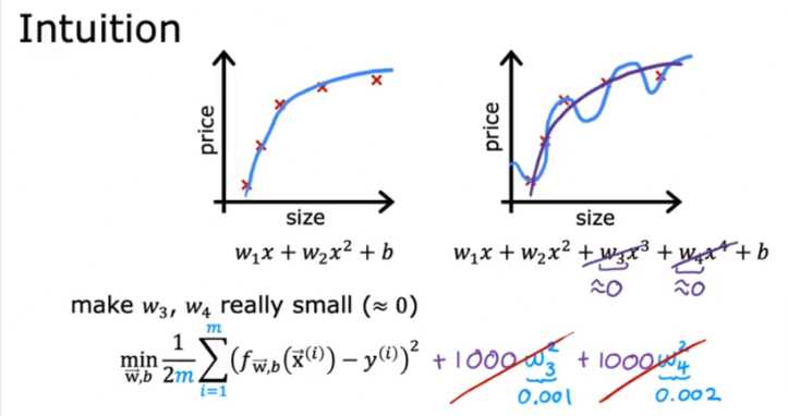
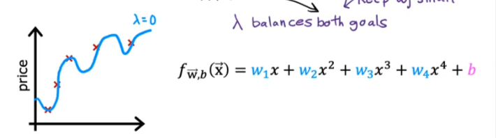
So basically we are taking a complex formula and simplifying it to a simple quadratic formula. So if we have thousands of features, we end up penalizing all the w values and minimizing their effect to make it a less wiggly curve and turn it into a smoother one.
So to penalize all the features we add a new term lambda “regularization parameter” to the equation
Linear Regression
Cost Function
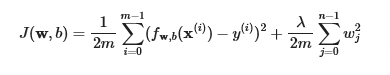
Previously the cost function was
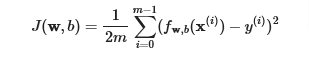
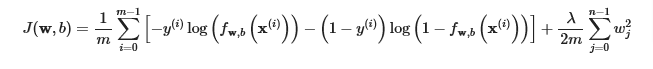
now we add the regularization parameter and we have, we scale by dividing into 2m to make it closer to earlier equation
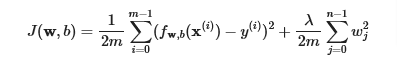
- The difference is the regularization term, λ2m∑j=0n−1wj2
- Including this term encourages gradient descent to minimize the size of the parameters. Note, in this example, the parameter b is not regularized. This is standard practice.
- Below is an implementation of equations (1) and (2). Note that this uses a standard pattern for this course, a
for loopover allmexamples. - We only use w and ignore b
Example
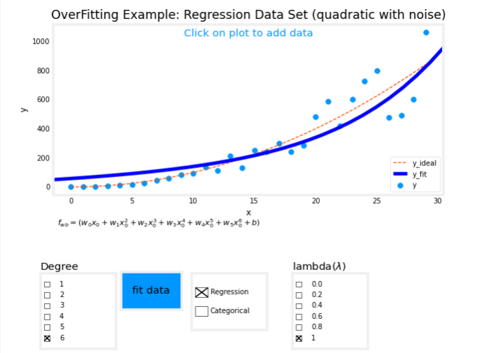
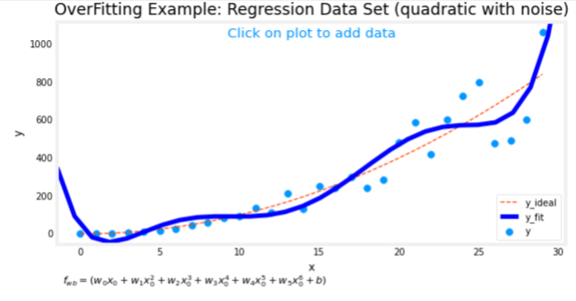
If Lambda = 0 we have this wiggly curve
If Lambda = 1010
In this case the algorithm will choose wi values to be close to zero to minimize their effect and therefore eliminating them and therefore our curve will be a straight line and underfits
Logistic Regression
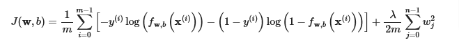
Cost Function
Gradient Descent
The algorithm does not change with regularization
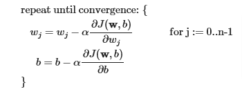
But the gradients will vary with regularization
The gradient calculation for both linear and logistic regression are nearly identical, differing only in computation of fwb.

Computing the Gradient with regularization (both linear/logistic)
The gradient calculation for both linear and logistic regression are nearly identical, differing only in computation of fwb.
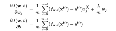
m is the number of training examples in the data set
fw,b(x(i)) is the model’s prediction, while y(i) is the target
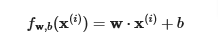
For a linear regression model
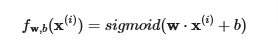
fw,b(x)=w⋅x+bFor a logistic regression model
z=w⋅x+b
fw,b(x)=g(z)
where g(z) is the sigmoid function:
g(z)=11+e−z
The term which adds regularization is the λmwj.
Code
.
Linear
def compute_cost_linear_reg(X, y, w, b, lambda_ = 1):
    """
    Computes the cost over all examples
    Args:
      X (ndarray (m,n): Data, m examples with n features
      y (ndarray (m,)): target values
      w (ndarray (n,)): model parameters
      b (scalar)      : model parameter
      lambda_ (scalar): Controls amount of regularization
    Returns:
      total_cost (scalar):  cost
    """

    m  = X.shape[0]
    n  = len(w)
    cost = 0.
    for i in range(m):
        f_wb_i = np.dot(X[i], w) + b                                   #(n,)(n,)=scalar, see np.dot
        cost = cost + (f_wb_i - y[i])**2                               #scalar
    cost = cost / (2 * m)                                              #scalar

    reg_cost = 0
    for j in range(n):
        reg_cost += (w[j]**2)                                          #scalar
    reg_cost = (lambda_/(2*m)) * reg_cost                              #scalar

    total_cost = cost + reg_cost                                       #scalar
    return total_cost
Calculate Cost
np.random.seed(1)
X_tmp = np.random.rand(5,6)
y_tmp = np.array([0,1,0,1,0])
w_tmp = np.random.rand(X_tmp.shape[1]).reshape(-1,)-0.5
b_tmp = 0.5
lambda_tmp = 0.7
cost_tmp = compute_cost_linear_reg(X_tmp, y_tmp, w_tmp, b_tmp, lambda_tmp)

print("Regularized cost:", cost_tmp)
Logistic
def compute_cost_logistic_reg(X, y, w, b, lambda_ = 1):
    """
    Computes the cost over all examples
    Args:
    Args:
      X (ndarray (m,n): Data, m examples with n features
      y (ndarray (m,)): target values
      w (ndarray (n,)): model parameters
      b (scalar)      : model parameter
      lambda_ (scalar): Controls amount of regularization
    Returns:
      total_cost (scalar):  cost
    """

    m,n  = X.shape
    cost = 0.
    for i in range(m):
        z_i = np.dot(X[i], w) + b                                      #(n,)(n,)=scalar, see np.dot
        f_wb_i = sigmoid(z_i)                                          #scalar
        cost +=  -y[i]*np.log(f_wb_i) - (1-y[i])*np.log(1-f_wb_i)      #scalar

    cost = cost/m                                                      #scalar

    reg_cost = 0
    for j in range(n):
        reg_cost += (w[j]**2)                                          #scalar
    reg_cost = (lambda_/(2*m)) * reg_cost                              #scalar

    total_cost = cost + reg_cost                                       #scalar
    return total_cost
Calculate Cost
np.random.seed(1)
X_tmp = np.random.rand(5,6)
y_tmp = np.array([0,1,0,1,0])
w_tmp = np.random.rand(X_tmp.shape[1]).reshape(-1,)-0.5
b_tmp = 0.5
lambda_tmp = 0.7
cost_tmp = compute_cost_logistic_reg(X_tmp, y_tmp, w_tmp, b_tmp, lambda_tmp)

print("Regularized cost:", cost_tmp)
Gradient Descent
Linear
def compute_gradient_linear_reg(X, y, w, b, lambda_):
    """
    Computes the gradient for linear regression
    Args:
      X (ndarray (m,n): Data, m examples with n features
      y (ndarray (m,)): target values
      w (ndarray (n,)): model parameters
      b (scalar)      : model parameter
      lambda_ (scalar): Controls amount of regularization

    Returns:
      dj_dw (ndarray (n,)): The gradient of the cost w.r.t. the parameters w.
      dj_db (scalar):       The gradient of the cost w.r.t. the parameter b.
    """
    m,n = X.shape           #(number of examples, number of features)
    dj_dw = np.zeros((n,))
    dj_db = 0.

    for i in range(m):
        err = (np.dot(X[i], w) + b) - y[i]
        for j in range(n):
            dj_dw[j] = dj_dw[j] + err * X[i, j]
        dj_db = dj_db + err
    dj_dw = dj_dw / m
    dj_db = dj_db / m

    for j in range(n):
        dj_dw[j] = dj_dw[j] + (lambda_/m) * w[j]

    return dj_db, dj_dw
Calculate w & b
np.random.seed(1)
X_tmp = np.random.rand(5,3)
y_tmp = np.array([0,1,0,1,0])
w_tmp = np.random.rand(X_tmp.shape[1])
b_tmp = 0.5
lambda_tmp = 0.7
dj_db_tmp, dj_dw_tmp =  compute_gradient_linear_reg(X_tmp, y_tmp, w_tmp, b_tmp, lambda_tmp)

print(f"dj_db: {dj_db_tmp}", )
print(f"Regularized dj_dw:\n {dj_dw_tmp.tolist()}", )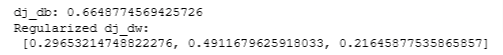
Logistic
def compute_gradient_logistic_reg(X, y, w, b, lambda_):
    """
    Computes the gradient for linear regression

    Args:
      X (ndarray (m,n): Data, m examples with n features
      y (ndarray (m,)): target values
      w (ndarray (n,)): model parameters
      b (scalar)      : model parameter
      lambda_ (scalar): Controls amount of regularization
    Returns
      dj_dw (ndarray Shape (n,)): The gradient of the cost w.r.t. the parameters w.
      dj_db (scalar)            : The gradient of the cost w.r.t. the parameter b.
    """
    m,n = X.shape
    dj_dw = np.zeros((n,))                            #(n,)
    dj_db = 0.0                                       #scalar

    for i in range(m):
        f_wb_i = sigmoid(np.dot(X[i],w) + b)          #(n,)(n,)=scalar
        err_i  = f_wb_i  - y[i]                       #scalar
        for j in range(n):
            dj_dw[j] = dj_dw[j] + err_i * X[i,j]      #scalar
        dj_db = dj_db + err_i
    dj_dw = dj_dw/m                                   #(n,)
    dj_db = dj_db/m                                   #scalar

    for j in range(n):
        dj_dw[j] = dj_dw[j] + (lambda_/m) * w[j]

return dj_db, dj_dw np.random.seed(1)
X_tmp = np.random.rand(5,3)
y_tmp = np.array([0,1,0,1,0])
w_tmp = np.random.rand(X_tmp.shape[1])
b_tmp = 0.5
lambda_tmp = 0.7
dj_db_tmp, dj_dw_tmp = compute_gradient_logistic_reg(X_tmp, y_tmp, w_tmp, b_tmp, lambda_tmp)
print(f"dj_db: {dj_db_tmp}", )
print(f"Regularized dj_dw:\n {dj_dw_tmp.tolist()}", )
Over-fit Example
plt.close("all")
display(output)
ofit = overfit_example(True)