import numpy as np
import matplotlib.pyplot as plt
plt.style.use('./deeplearning.mplstyle')
import tensorflow as tf
from tensorflow.keras.models import Sequential
from tensorflow.keras.layers import Dense
from lab_utils_common import dlc
from lab_coffee_utils import load_coffee_data, plt_roast, plt_prob, plt_layer, plt_network, plt_output_unit
import logging
logging.getLogger("tensorflow").setLevel(logging.ERROR)
tf.autograph.set_verbosity(0)NN in TF - Coffee Roasting
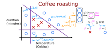
Let’s put the coffee roasting example covered in the discussoin pages all together in code, so let’s build a small NN using Tensorflow
If you remember, here is what we discussed earlier
Setup
.
Dataset
- As you see we have a 200 rows and 2 columns as input Features in X
- One column 200 rows as Target in Y
X,Y = load_coffee_data();
print(X.shape, Y.shape)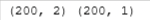
View
- Remember X is for Good Roast
- O for Bad Roast
plt_roast(X,Y)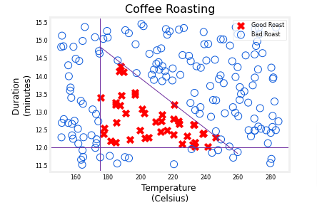
Normalize Data
As we covered in previous pages, let’s normalize the data to have similar range which will make the process go faster.
We will use a Keras normalization layer
- create a “Normalization Layer”. Note, as applied here, this is not a layer in your model.
- ‘adapt’ the data. This learns the mean and variance of the data set and saves the values internally.
- normalize the data
- It is important to apply normalization to any future data that utilizes the learned model.
print(f"Temperature Max, Min pre normalization: {np.max(X[:,0]):0.2f}, {np.min(X[:,0]):0.2f}")
print(f"Duration    Max, Min pre normalization: {np.max(X[:,1]):0.2f}, {np.min(X[:,1]):0.2f}")
norm_l = tf.keras.layers.Normalization(axis=-1)
norm_l.adapt(X)  # learns mean, variance
Xn = norm_l(X)
print(f"Temperature Max, Min post normalization: {np.max(Xn[:,0]):0.2f}, {np.min(Xn[:,0]):0.2f}")
print(f"Duration    Max, Min post normalization: {np.max(Xn[:,1]):0.2f}, {np.min(Xn[:,1]):0.2f}")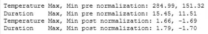
Tile Data
Tile data to increase the training set size and reduce the number of training epochs
- Instead of 200 rows we now have 200,000 rows
Xt = np.tile(Xn,(1000,1))
Yt= np.tile(Y,(1000,1))
print(Xt.shape, Yt.shape) 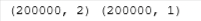
Build TF Model
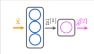
- Let’s build the model we’ve talked about before
- Let’s start by setting the seed so we can replicate the results
- Note 1: The
tf.keras.Input(shape=(2,)),specifies the expected shape of the input. This allows Tensorflow to size the weights and bias parameters at this point. This is useful when exploring Tensorflow models. This statement can be omitted in practice and Tensorflow will size the network parameters when the input data is specified in themodel.fitstatement.
Note 2: Including the sigmoid activation in the final layer is not considered best practice. It would instead be accounted for in the loss which improves numerical stability.
tf.random.set_seed(1234)  # applied to achieve consistent results
model = Sequential(
    [
        tf.keras.Input(shape=(2,)),
        Dense(3, activation='sigmoid', name = 'layer1'),
        Dense(1, activation='sigmoid', name = 'layer2')
     ]
)
Preview
- The model.summary() provides a description of the network we just defined
model.summary()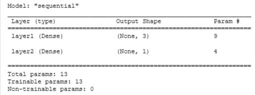
- The parameter counts shown in the summary correspond to the number of elements in the weight and bias arrays as shown below.
L1_num_params = 2 * 3 + 3   # W1 parameters  + b1 parameters
L2_num_params = 3 * 1 + 1   # W2 parameters  + b2 parameters
print("L1 params = ", L1_num_params, ", L2 params = ", L2_num_params  )
Preview Weights
Let’s examine the weights and biases Tensorflow has instantiated. The weights 𝑊W should be of size (number of features in input, number of units in the layer) while the bias 𝑏b size should match the number of units in the layer:
- In the first layer with 3 units, we expect W to have a size of (2,3) and 𝑏b should have 3 elements.
- In the second layer with 1 unit, we expect W to have a size of (3,1) and 𝑏b should have 1 element.
W1, b1 = model.get_layer("layer1").get_weights()
W2, b2 = model.get_layer("layer2").get_weights()
print(f"W1{W1.shape}:\n", W1, f"\nb1{b1.shape}:", b1)
print(f"W2{W2.shape}:\n", W2, f"\nb2{b2.shape}:", b2)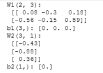
Compile & Train
- The
model.compilestatement defines a loss function and specifies a compile optimization. - The
model.fitstatement runs gradient descent and fits the weights to the data.
model.compile(
    loss = tf.keras.losses.BinaryCrossentropy(),
    optimizer = tf.keras.optimizers.Adam(learning_rate=0.01),
)

model.fit(
    Xt,Yt,
    epochs=10,
)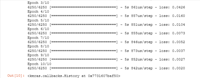
Epochs and batches
In the fit statement above, the number of epochs was set to 10. This specifies that the entire data set should be applied during training 10 times. During training, you see output describing the progress of training that looks like this:
Epoch 1/10 6250/6250 [==============================] - 6s 910us/step - loss: 0.1782The first line, Epoch 1/10, describes which epoch the model is currently running. For efficiency, the training data set is broken into ‘batches’. The default size of a batch in Tensorflow is 32. There are 200000 examples in our expanded data set or 6250 batches. The notation on the 2nd line 6250/6250 [==== is describing which batch has been executed.
Updated Weights
After fitting, the weights have been updated:
W1, b1 = model.get_layer("layer1").get_weights()
W2, b2 = model.get_layer("layer2").get_weights()
print("W1:\n", W1, "\nb1:", b1)
print("W2:\n", W2, "\nb2:", b2)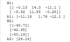
You can see that the values are different from what you printed before calling model.fit(). With these, the model should be able to discern what is a good or bad coffee roast.
For the purpose of the next discussion, instead of using the weights you got right away, you will first set some weights we saved from a previous training run. Different training runs can produce somewhat different results and the following discussion applies when the model has the weights you will load below.
Feel free to re-run the notebook later with the cell below commented out to see if there is any difference. If you got a low loss after the training above (e.g. 0.002), then you will most likely get the same results.
# After finishing the lab later, you can re-run all
# cells except this one to see if your trained model
# gets the same results.

# Set weights from a previous run.
W1 = np.array([
    [-8.94,  0.29, 12.89],
    [-0.17, -7.34, 10.79]] )
b1 = np.array([-9.87, -9.28,  1.01])
W2 = np.array([
    [-31.38],
    [-27.86],
    [-32.79]])
b2 = np.array([15.54])

# Replace the weights from your trained model with
# the values above.
model.get_layer("layer1").set_weights([W1,b1])
model.get_layer("layer2").set_weights([W2,b2])
# Check if the weights are successfully replaced
W1, b1 = model.get_layer("layer1").get_weights()
W2, b2 = model.get_layer("layer2").get_weights()
print("W1:\n", W1, "\nb1:", b1)
print("W2:\n", W2, "\nb2:", b2)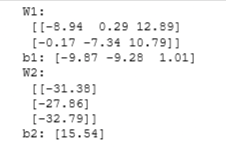
Predictions
Once you have a trained model, you can then use it to make predictions. Recall that the output of our model is a probability. In this case, the probability of a good roast. To make a decision, one must apply the probability to a threshold. In this case, we will use 0.5
Create Input
- The model is expecting one or more examples where examples are in the rows of matrix.
- In this case, we have two features so the matrix will be (m,2) where m is the number of examples.
- Recall, we have normalized the input features so we must normalize our test data as well.
- To make a prediction, you apply the
predictmethod.
X_test = np.array([
    [200,13.9],  # positive example
    [200,17]])   # negative example
X_testn = norm_l(X_test)
predictions = model.predict(X_testn)
print("predictions = \n", predictions)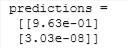
Convert to Probability
# Apply a threshold
yhat = np.zeros_like(predictions)
for i in range(len(predictions)):
    if predictions[i] >= 0.5:
        yhat[i] = 1
    else:
        yhat[i] = 0
print(f"decisions = \n{yhat}")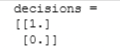
or use
yhat = (predictions >= 0.5).astype(int)
print(f"decisions = \n{yhat}")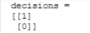
Dissect Layers
Let’s examine the functions of the units to determine their role in the coffee roasting decision.
- We will plot the output of each node for all values of the inputs (duration,temp).
- Each unit is a logistic function whose output can range from zero to one.
- The shading in the graph represents the output value.
plt_layer(X,Y.reshape(-1,),W1,b1,norm_l)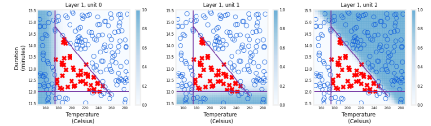
The shading shows that each unit is responsible for a different “bad roast” region. unit 0 has larger values when the temperature is too low. unit 1 has larger values when the duration is too short and unit 2 has larger values for bad combinations of time/temp. It is worth noting that the network learned these functions on its own through the process of gradient descent. They are very much the same sort of functions a person might choose to make the same decisions.
The function plot of the final layer is a bit more difficult to visualize. It’s inputs are the output of the first layer. We know that the first layer uses sigmoids so their output range is between zero and one. We can create a 3-D plot that calculates the output for all possible combinations of the three inputs. This is shown below. Above, high output values correspond to ‘bad roast’ area’s. Below, the maximum output is in area’s where the three inputs are small values corresponding to ‘good roast’ area’s.
plt_output_unit(W2,b2)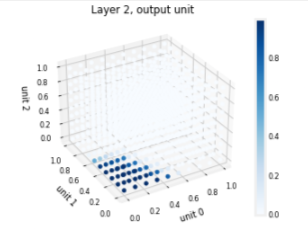
The final graph shows the whole network in action.
The left graph is the raw output of the final layer represented by the blue shading. This is overlaid on the training data represented by the X’s and O’s.
The right graph is the output of the network after a decision threshold. The X’s and O’s here correspond to decisions made by the network.
The following takes a moment to run
netf= lambda x : model.predict(norm_l(x))
plt_network(X,Y,netf)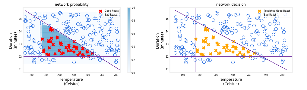
Functions
Here are the functions used
def load_coffee_data():
    """ Creates a coffee roasting data set.
        roasting duration: 12-15 minutes is best
        temperature range: 175-260C is best
    """
    rng = np.random.default_rng(2)
    X = rng.random(400).reshape(-1,2)
    X[:,1] = X[:,1] * 4 + 11.5          # 12-15 min is best
    X[:,0] = X[:,0] * (285-150) + 150  # 350-500 F (175-260 C) is best
    Y = np.zeros(len(X))

    i=0
    for t,d in X:
        y = -3/(260-175)*t + 21
        if (t > 175 and t < 260 and d > 12 and d < 15 and d<=y ):
            Y[i] = 1
        else:
            Y[i] = 0
        i += 1

    return (X, Y.reshape(-1,1))
def plt_roast(X,Y):
Y = Y.reshape(-1,)
colormap = np.array(['r', 'b'])
fig, ax = plt.subplots(1,1,)
ax.scatter(X[Y==1,0],X[Y==1,1], s=70, marker='x', c='red', label="Good Roast" )
ax.scatter(X[Y==0,0],X[Y==0,1], s=100, marker='o', facecolors='none',
edgecolors=dlc["dldarkblue"],linewidth=1, label="Bad Roast")
tr = np.linspace(175,260,50)
ax.plot(tr, (-3/85) * tr + 21, color=dlc["dlpurple"],linewidth=1)
ax.axhline(y=12,color=dlc["dlpurple"],linewidth=1)
ax.axvline(x=175,color=dlc["dlpurple"],linewidth=1)
ax.set_title(f"Coffee Roasting", size=16)
ax.set_xlabel("Temperature \n(Celsius)",size=12)
ax.set_ylabel("Duration \n(minutes)",size=12)
ax.legend(loc='upper right')
plt.show()