import numpy as np
%matplotlib widget
import matplotlib.pyplot as plt
from lab_utils_common import plot_data, sigmoid, draw_vthresh
plt.style.use('./deeplearning.mplstyle')Decision Boundary
So how is our decision model computing the two classes. How does it know when to choose one or the other?
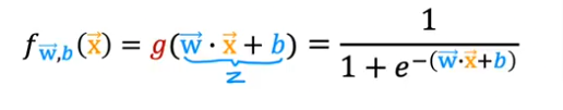
Remember the sigmoid function is defined as
So to predict which one is 0 or 1, we set a threshold above which it is 1 and below it is 0. But how do we relate that to the value of z, so we can make the formula simpler without introducing a new variable being the threshold. How do we relate threshold to z?
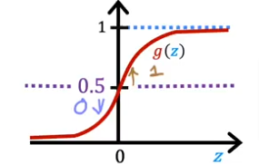
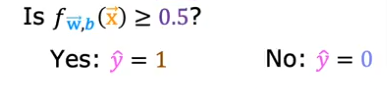
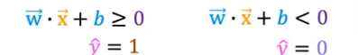
- So if we substitue g(z) for F then, when will g(z) >= 0.5, as you see from the plot, it is at 0.5 when z=0.
- In other words, when w.x+b>=0 then the predicted value is 1
- when w.x+b<0 then predicted value is 0
Two Features
Linear DB
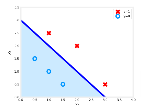
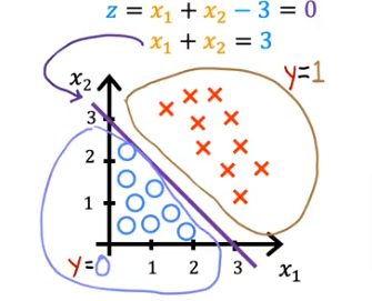
- Let’s pretend we have two features instead x1 and x2 and we plot it and see the actual y values as shown.
- So when would our model predict 1 or 0?
- well if you remember from above we are looking for when which is the decision boundary
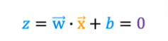
- that’s our threshold
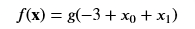
- So let’s say our model came up with w1=1, w2=1, b=-3 as the optimal values from gradient descent
- So when would our z=0 with those values?
- Well the formula would be
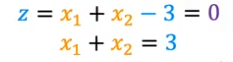
- and when would that be true? Well when x1=0 then x2=3 and when x1=3 & x2=0
- so draw a line at those points and we get
Non-Linear DB
- Let’s look at it when our decision boundary is not a straight line
- Let’s use a polynomial formula below
- the DB is still when z=0
- evaluate the formula and you get where the boundary is
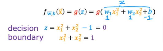
- if we plot it you’ll see an eclipse around the 0 point at center and radius of 1
- anything outside the circle is 1 and inside is 0

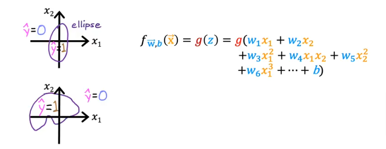
Higher Oder Polynomial
Would present more complicated decision boundaries.
Code
Setup
.
Dataset
Let’s suppose you have following training dataset
- The input variable
Xis a numpy array which has 6 training examples, each with two features - The output variable
yis also a numpy array with 6 examples, andyis either0or1
X = np.array([[0.5, 1.5], [1,1], [1.5, 0.5], [3, 0.5], [2, 2], [1, 2.5]])
y = np.array([0, 0, 0, 1, 1, 1]).reshape(-1,1)
Plot Data
fig,ax = plt.subplots(1,1,figsize=(4,4))
plot_data(X, y, ax)

ax.axis([0, 4, 0, 3.5])
ax.set_ylabel('$x_1$')
ax.set_xlabel('$x_0$')
plt.show()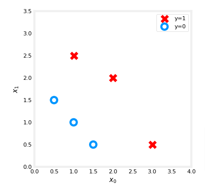
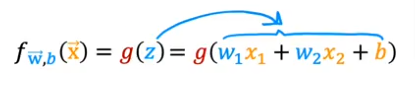
- Remember the logistic regression model
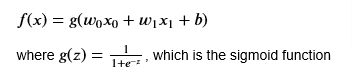
- Let’s say you trained the model and you arrived at b=-3, w0=1, w1=1
- If you remember the vector representation would be
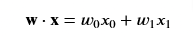
Sigmoid
def sigmoid(z):
    """
    Compute the sigmoid of z

    Parameters
    ----------
    z : array_like
        A scalar or numpy array of any size.

    Returns
    -------
     g : array_like
         sigmoid(z)
    """
    z = np.clip( z, -500, 500 )           # protect against overflow
    g = 1.0/(1.0+np.exp(-z))

    return g
Plot Sigmoid
- So far we’ve covered all this in the previous page
# Plot sigmoid(z) over a range of values from -10 to 10
z = np.arange(-10,11)

fig,ax = plt.subplots(1,1,figsize=(5,3))
# Plot z vs sigmoid(z)
ax.plot(z, sigmoid(z), c="b")

ax.set_title("Sigmoid function")
ax.set_ylabel('sigmoid(z)')
ax.set_xlabel('z')
draw_vthresh(ax,0)
Decision Boundary
Using the parameter values we arrived at and listed earlier let’s see what our logistic model will show as the boundary
# Choose values between 0 and 6
x0 = np.arange(0,6)

x1 = 3 - x0
fig,ax = plt.subplots(1,1,figsize=(5,4))
# Plot the decision boundary
ax.plot(x0,x1, c="b")
ax.axis([0, 4, 0, 3.5])

# Fill the region below the line
ax.fill_between(x0,x1, alpha=0.2)

# Plot the original data
plot_data(X,y,ax)
ax.set_ylabel(r'$x_1$')
ax.set_xlabel(r'$x_0$')
plt.show()