import numpy as np
import matplotlib.pyplot as plt
from utils import *
import copy
import math

#%matplotlib inlineAdmission Prediction
Problem Statement
Suppose that you are the administrator of a university department and you want to determine each applicant’s chance of admission based on their results on two exams.
- You have historical data from previous applicants that you can use as a training set for logistic regression.
- For each training example, you have the applicant’s scores on two exams and the admissions decision.
- Your task is to build a classification model that estimates an applicant’s probability of admission based on the scores from those two exams.
Setup
.
Data
You will start by loading the dataset for this task.
- The
load_dataset()function shown below loads the data into variablesX_trainandy_trainX_traincontains exam scores on two exams for a studenty_trainis the admission decisiony_train = 1if the student was admittedy_train = 0if the student was not admitted
Both
X_trainandy_trainare numpy arrays.
def load_data():
    data = np.loadtxt("data/ex2data1.txt", delimiter=',')
    X = data[:,0]  # all of column 1
    y = data[:,1]  # all of column 2
    return X, y
# load dataset
X_train, y_train = load_data()View Data
print("First five elements in X_train are:\n", X_train[:5])
print("Type of X_train:",type(X_train))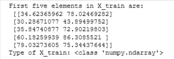
print("First five elements in y_train are:\n", y_train[:5])
print("Type of y_train:",type(y_train))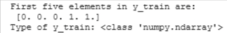
print ('The shape of X_train is: ' + str(X_train.shape))
print ('The shape of y_train is: ' + str(y_train.shape))
print ('We have m = %d training examples' % (len(y_train)))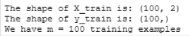
# Plot examples
plot_data(X_train, y_train[:], pos_label="Admitted", neg_label="Not admitted")

# Set the y-axis label
plt.ylabel('Exam 2 score')
# Set the x-axis label
plt.xlabel('Exam 1 score')
plt.legend(loc="upper right")
plt.show()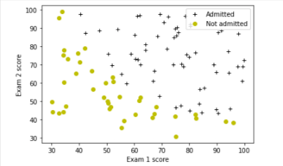
Let’s build a logistic regression model to fit this data
Sigmoid Function
Calculate Sigmoid
def sigmoid(z):
    """
    Compute the sigmoid of z

    Args:
        z (ndarray): A scalar, numpy array of any size.

    Returns:
        g (ndarray): sigmoid(z), with the same shape as z

    """

    g = 1/(1+np.exp(-z))

    return g
Check Value
# Note: You can edit this value
value = 0

print (f"sigmoid({value}) = {sigmoid(value)}")
value = 2.5

print (f"sigmoid({value}) = {sigmoid(value)}")
Check with Vector
print ("sigmoid([ -1, 0, 1, 2]) = " + str(sigmoid(np.array([-1, 0, 1, 2]))))

# UNIT TESTS
from public_tests import *
sigmoid_test(sigmoid)
Cost Function
Cost function is
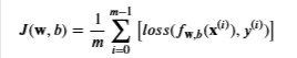
- m is the number of training examples in the dataset
- Loss is the cost for a single data point

- first part is the model prediction, while y(i) is the actual label
- g is the sigmoid function
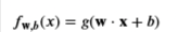
- It might be helpful to first calculate an intermediate variable 𝑧𝐰,𝑏(𝐱(𝑖))=𝐰⋅𝐱(𝐢)+𝑏=𝑤0𝑥(𝑖)0+…+𝑤𝑛−1𝑥(𝑖)𝑛−1+𝑏zw,b(x(i))=w⋅x(i)+b=w0x0(i)+…+wn−1xn−1(i)+b where 𝑛n is the number of features, before calculating 𝑓𝐰,𝑏(𝐱(𝑖))=𝑔(𝑧𝐰,𝑏(𝐱(𝑖)))
Note:
As you are doing this, remember that the variables
X_trainandy_trainare not scalar values but matrices of shape (𝑚,𝑛m,n) and (𝑚𝑚,1) respectively, where 𝑛𝑛 is the number of features and 𝑚𝑚 is the number of training examples.You can use the sigmoid function that you implemented above for this part.
def compute_cost(X, y, w, b, *argv):
    """
    Computes the cost over all examples
    Args:
      X : (ndarray Shape (m,n)) data, m examples by n features
      y : (ndarray Shape (m,))  target value
      w : (ndarray Shape (n,))  values of parameters of the model
      b : (scalar)              value of bias parameter of the model
      *argv : unused, for compatibility with regularized version below
    Returns:
      total_cost : (scalar) cost
    """

    m, n = X.shape


    loss_sum = 0

    # Loop over each training example
    for i in range(m):

        # First calculate z_wb = w[0]*X[i][0]+...+w[n-1]*X[i][n-1]+b
        z_wb = 0
        # Loop over each feature
        for j in range(n):
            # Add the corresponding term to z_wb
            z_wb_ij = w[j] * X[i,j] # Your code here to calculate w[j] * X[i][j]
            z_wb += z_wb_ij # equivalent to z_wb = z_wb + z_wb_ij
        # Add the bias term to z_wb
        z_wb += b # equivalent to z_wb = z_wb + b

        f_wb = sigmoid(z_wb) # Your code here to calculate prediction f_wb for a training example
        loss =  -y[i] * np.log(f_wb) - (1- y[i]) * np.log(1-f_wb) # Your code here to calculate loss for a training example

        loss_sum += loss # equivalent to loss_sum = loss_sum + loss

    total_cost = (1 / m) * loss_sum


    return total_cost
Check Values
# Compute and display cost with non-zero w and b
test_w = np.array([0.2, 0.2])
test_b = -24.
cost = compute_cost(X_train, y_train, test_w, test_b)

print('Cost at test w and b (non-zeros): {:.3f}'.format(cost))


# UNIT TESTS
compute_cost_test(compute_cost)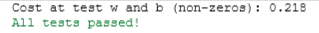
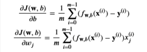
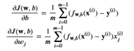
Gradient
Recall the gradient descent is
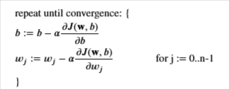
Create a function to compute the gradient
def compute_gradient(X, y, w, b, *argv):
    """
    Computes the gradient for logistic regression

    Args:
      X : (ndarray Shape (m,n)) data, m examples by n features
      y : (ndarray Shape (m,))  target value
      w : (ndarray Shape (n,))  values of parameters of the model
      b : (scalar)              value of bias parameter of the model
      *argv : unused, for compatibility with regularized version below
    Returns
      dj_dw : (ndarray Shape (n,)) The gradient of the cost w.r.t. the parameters w.
      dj_db : (scalar)             The gradient of the cost w.r.t. the parameter b.
    """
    m, n = X.shape
    dj_dw = np.zeros(w.shape)
    dj_db = 0.


    for i in range(m):
        # Calculate z_wb like we did above in compute_cost function
        z_wb = 0
        for j in range(n):
            z_wb_ij = w[j] * X[i,j] # Your code here to calculate w[j] * X[i][j]
            z_wb += z_wb_ij

        z_wb += b  # add the bias term

        f_wb = sigmoid(z_wb) # Your code here to calculate prediction f_wb for a training example

        # so far it's the same code used in the cost function

        dj_db_i = f_wb - y[i]
        dj_db += dj_db_i

        for j in range(n):
            dj_dw_ij = (f_wb-y[i]) * X[i][j]
            dj_dw[j] += dj_dw_ij

    dj_dw = dj_dw/m
    dj_db = dj_db/m


    return dj_db, dj_dw
Check Values
# Compute and display gradient with w and b initialized to zeros
initial_w = np.zeros(n)
initial_b = 0.

dj_db, dj_dw = compute_gradient(X_train, y_train, initial_w, initial_b)
print(f'dj_db at initial w and b (zeros):{dj_db}' )
print(f'dj_dw at initial w and b (zeros):{dj_dw.tolist()}' )
Display Cost
# Compute and display cost and gradient with non-zero w and b
test_w = np.array([ 0.2, -0.5])
test_b = -24
dj_db, dj_dw  = compute_gradient(X_train, y_train, test_w, test_b)

print('dj_db at test w and b:', dj_db)
print('dj_dw at test w and b:', dj_dw.tolist())

# UNIT TESTS
compute_gradient_test(compute_gradient)
Gradient Descent
Let’s find the optimal parameters of a logistic regression model by using gradient descent
- A good way to verify that gradient descent is working correctly is to look at the value of 𝐽(𝐰,𝑏)J(w,b) and check that it is decreasing with each step.
- Assuming you have implemented the gradient and computed the cost correctly, your value of 𝐽(𝐰,𝑏)J(w,b) should never increase, and should converge to a steady value by the end of the algorithm.
def gradient_descent(X, y, w_in, b_in, cost_function, gradient_function, alpha, num_iters, lambda_):
    """
    Performs batch gradient descent to learn theta. Updates theta by taking
    num_iters gradient steps with learning rate alpha

    Args:
      X :    (ndarray Shape (m, n) data, m examples by n features
      y :    (ndarray Shape (m,))  target value
      w_in : (ndarray Shape (n,))  Initial values of parameters of the model
      b_in : (scalar)              Initial value of parameter of the model
      cost_function :              function to compute cost
      gradient_function :          function to compute gradient
      alpha : (float)              Learning rate
      num_iters : (int)            number of iterations to run gradient descent
      lambda_ : (scalar, float)    regularization constant

    Returns:
      w : (ndarray Shape (n,)) Updated values of parameters of the model after
          running gradient descent
      b : (scalar)                Updated value of parameter of the model after
          running gradient descent
    """

    # number of training examples
    m = len(X)

    # An array to store cost J and w's at each iteration primarily for graphing later
    J_history = []
    w_history = []

    for i in range(num_iters):

        # Calculate the gradient and update the parameters
        dj_db, dj_dw = gradient_function(X, y, w_in, b_in, lambda_)

        # Update Parameters using w, b, alpha and gradient
        w_in = w_in - alpha * dj_dw
        b_in = b_in - alpha * dj_db

        # Save cost J at each iteration
        if i<100000:      # prevent resource exhaustion
            cost =  cost_function(X, y, w_in, b_in, lambda_)
            J_history.append(cost)

        # Print cost every at intervals 10 times or as many iterations if < 10
        if i% math.ceil(num_iters/10) == 0 or i == (num_iters-1):
            w_history.append(w_in)
            print(f"Iteration {i:4}: Cost {float(J_history[-1]):8.2f}   ")

    return w_in, b_in, J_history, w_history #return w and J,w history for graphing
Run GD to learn the parameters for our dataset
np.random.seed(1)
initial_w = 0.01 * (np.random.rand(2) - 0.5)
initial_b = -8

# Some gradient descent settings
iterations = 10000
alpha = 0.001

w,b, J_history,_ = gradient_descent(X_train ,y_train, initial_w, initial_b,
                                   compute_cost, compute_gradient, alpha, iterations, 0)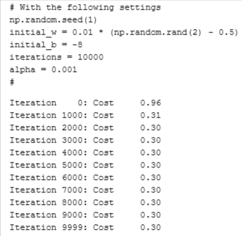
Decision Boundary
We will use a helper in utils.py to plot it
plot_decision_boundary(w, b, X_train, y_train)
# Set the y-axis label
plt.ylabel('Exam 2 score')
# Set the x-axis label
plt.xlabel('Exam 1 score')
plt.legend(loc="upper right")
plt.show()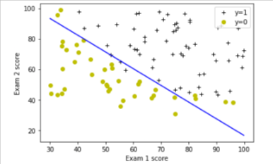
Predict Function
We can evaluate the quality of the parameters we have found by seeing how well the learned model predicts on our training set.
You will implement the predict function below to do this.
We will implement a predict function to produce 1 or 0 predictions given a dataset and a learned parameter vector w and b
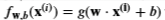
First you need to compute the prediction from the model 𝑓(𝑥(𝑖))=𝑔(𝑤⋅𝑥(𝑖)+𝑏)f(x(i))=g(w⋅x(i)+b) for every example
- You’ve implemented this before in the parts above
We interpret the output of the model (𝑓(𝑥(𝑖))f(x(i))) as the probability that 𝑦(𝑖)=1y(i)=1 given 𝑥(𝑖)x(i) and parameterized by 𝑤w.
Therefore, to get a final prediction (𝑦(𝑖)=0y(i)=0 or 𝑦(𝑖)=1y(i)=1) from the logistic regression model, you can use the following heuristic -
if 𝑓(𝑥(𝑖))>=0.5f(x(i))>=0.5, predict 𝑦(𝑖)=1y(i)=1
if 𝑓(𝑥(𝑖))<0.5f(x(i))<0.5, predict 𝑦(𝑖)=0y(i)=0
If you get stuck, you can check out the hints presented after the cell below to help you with the implementation.
def predict(X, w, b):
    """
    Predict whether the label is 0 or 1 using learned logistic
    regression parameters w

    Args:
      X : (ndarray Shape (m,n)) data, m examples by n features
      w : (ndarray Shape (n,))  values of parameters of the model
      b : (scalar)              value of bias parameter of the model

    Returns:
      p : (ndarray (m,)) The predictions for X using a threshold at 0.5
    """
    # number of training examples
    m, n = X.shape
    p = np.zeros(m)

    ### START CODE HERE ###
    # Loop over each example
    for i in range(m):
        z_wb = 0
        # Loop over each feature
        for j in range(n):
            # Add the corresponding term to z_wb
            z_wb_ij = w[j] * X[i][j]
            z_wb += z_wb_ij

        # Add bias term
        z_wb += b

        # Calculate the prediction for this example
        f_wb = sigmoid(z_wb)

        # Apply the threshold
        p[i] = f_wb >= 0.5

    ### END CODE HERE ###
    return p
Check Accuracy
# Test your predict code
np.random.seed(1)
tmp_w = np.random.randn(2)
tmp_b = 0.3
tmp_X = np.random.randn(4, 2) - 0.5

tmp_p = predict(tmp_X, tmp_w, tmp_b)
print(f'Output of predict: shape {tmp_p.shape}, value {tmp_p}')

# UNIT TESTS
predict_test(predict)
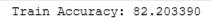
#Compute accuracy on our training set
p = predict(X_train, w,b)
print('Train Accuracy: %f'%(np.mean(p == y_train) * 100))
Regularized Logistic
Predict whether microchips from a fabrication plant passes quality assurance.
# load dataset
X_train, y_train = load_data("data/ex2data2.txt")
# print X_train
print("X_train:", X_train[:5])
print("Type of X_train:",type(X_train))
# print y_train
print("y_train:", y_train[:5])
print("Type of y_train:",type(y_train))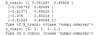
print ('The shape of X_train is: ' + str(X_train.shape))
print ('The shape of y_train is: ' + str(y_train.shape))
print ('We have m = %d training examples' % (len(y_train)))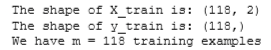
# Plot examples
plot_data(X_train, y_train[:], pos_label="Accepted", neg_label="Rejected")

# Set the y-axis label
plt.ylabel('Microchip Test 2')
# Set the x-axis label
plt.xlabel('Microchip Test 1')
plt.legend(loc="upper right")
plt.show()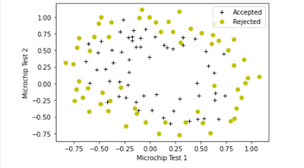
Figure shows that our dataset cannot be separated into positive and negative examples by a straight-line through the plot. Therefore, a straight forward application of logistic regression will not perform well on this dataset since logistic regression will only be able to find a linear decision boundary.
Map Features
One way to fit the data better is to create more features from each data point. In the provided function map_feature, we will map the features into all polynomial terms of x1 and x2 up to the sixth power.
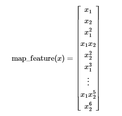
As a result of this mapping, our vector of two features (the scores on two QA tests) has been transformed into a 27-dimensional vector.
A logistic regression classifier trained on this higher-dimension feature vector will have a more complex decision boundary and will be nonlinear when drawn in our 2-dimensional plot.
We have provided the
map_featurefunction for you in utils.py.
print("Original shape of data:", X_train.shape)

mapped_X =  map_feature(X_train[:, 0], X_train[:, 1])
print("Shape after feature mapping:", mapped_X.shape)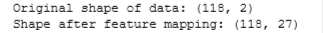
print("X_train[0]:", X_train[0])
print("mapped X_train[0]:", mapped_X[0])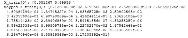
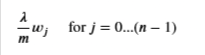
Remember the Cost function for regularized logistic regression
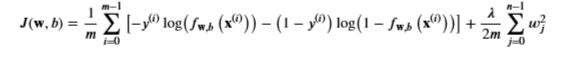
with the difference from the non-regularized function is the far right term
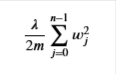
Regularized Cost Function
def compute_cost_reg(X, y, w, b, lambda_ = 1):
    """
    Computes the cost over all examples
    Args:
      X : (ndarray Shape (m,n)) data, m examples by n features
      y : (ndarray Shape (m,))  target value
      w : (ndarray Shape (n,))  values of parameters of the model
      b : (scalar)              value of bias parameter of the model
      lambda_ : (scalar, float) Controls amount of regularization
    Returns:
      total_cost : (scalar)     cost
    """

    m, n = X.shape

    # Calls the compute_cost function that you implemented above
    cost_without_reg = compute_cost(X, y, w, b)

    # You need to calculate this value
    reg_cost = 0.


    reg_cost = 0
    for j in range(n):
        reg_cost += (w[j]**2)                                          #scalar
    reg_cost = (lambda_/(2*m)) * reg_cost


    # Add the regularization cost to get the total cost
    total_cost = cost_without_reg + reg_cost

    return total_cost
Check Value
X_mapped = map_feature(X_train[:, 0], X_train[:, 1])
np.random.seed(1)
initial_w = np.random.rand(X_mapped.shape[1]) - 0.5
initial_b = 0.5
lambda_ = 0.5
cost = compute_cost_reg(X_mapped, y_train, initial_w, initial_b, lambda_)

print("Regularized cost :", cost)

# UNIT TEST
compute_cost_reg_test(compute_cost_reg)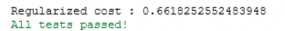
Gradient Regularized
We already implemented this above
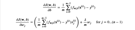
With the difference being
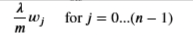
Gradient Regularized
- Add the parameter below to the compute_gradient from earlier
def compute_gradient_reg(X, y, w, b, lambda_ = 1):
    """
    Computes the gradient for logistic regression with regularization

    Args:
      X : (ndarray Shape (m,n)) data, m examples by n features
      y : (ndarray Shape (m,))  target value
      w : (ndarray Shape (n,))  values of parameters of the model
      b : (scalar)              value of bias parameter of the model
      lambda_ : (scalar,float)  regularization constant
    Returns
      dj_db : (scalar)             The gradient of the cost w.r.t. the parameter b.
      dj_dw : (ndarray Shape (n,)) The gradient of the cost w.r.t. the parameters w.

    """
    m, n = X.shape

    dj_db, dj_dw = compute_gradient(X, y, w, b)

    for j in range(n):
        dj_dw[j] = dj_dw[j] + (lambda_/m) * w[j]

    return dj_db, dj_dw
X_mapped = map_feature(X_train[:, 0], X_train[:, 1])
np.random.seed(1)
initial_w = np.random.rand(X_mapped.shape[1]) - 0.5
initial_b = 0.5
lambda_ = 0.5
dj_db, dj_dw = compute_gradient_reg(X_mapped, y_train, initial_w, initial_b, lambda_)
print(f"dj_db: {dj_db}", )
print(f"First few elements of regularized dj_dw:\n {dj_dw[:4].tolist()}", )
# UNIT TESTS
compute_gradient_reg_test(compute_gradient_reg)
Learn Using GD
# Initialize fitting parameters
np.random.seed(1)
initial_w = np.random.rand(X_mapped.shape[1])-0.5
initial_b = 1.

# Set regularization parameter lambda_ (you can try varying this)
lambda_ = 0.01

# Some gradient descent settings
iterations = 10000
alpha = 0.01

w,b, J_history,_ = gradient_descent(X_mapped, y_train, initial_w, initial_b,
                                    compute_cost_reg, compute_gradient_reg,
                                    alpha, iterations, lambda_)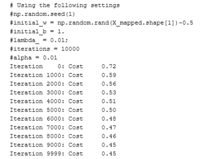
Plot Decision Bounday
To help you visualize the model learned by this classifier, we will use our plot_decision_boundary function which plots the (non-linear) decision boundary that separates the positive and negative examples.
In the function, we plotted the non-linear decision boundary by computing the classifier’s predictions on an evenly spaced grid and then drew a contour plot of where the predictions change from y = 0 to y = 1.
After learning the parameters 𝑤w,𝑏b, the next step is to plot a decision boundary similar to Figure 4.
plot_decision_boundary(w, b, X_mapped, y_train)
# Set the y-axis label
plt.ylabel('Microchip Test 2')
# Set the x-axis label
plt.xlabel('Microchip Test 1')
plt.legend(loc="upper right")
plt.show()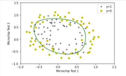
Evaluate Logistic Regression Model
#Compute accuracy on the training set
p = predict(X_mapped, w, b)

print('Train Accuracy: %f'%(np.mean(p == y_train) * 100))