import numpy as np
%matplotlib widget
import matplotlib.pyplot as plt
from plt_logistic_loss import  plt_logistic_cost, plt_two_logistic_loss_curves, plt_simple_example
from plt_logistic_loss import soup_bowl, plt_logistic_squared_error
plt.style.use('./deeplearning.mplstyle')Cost Function
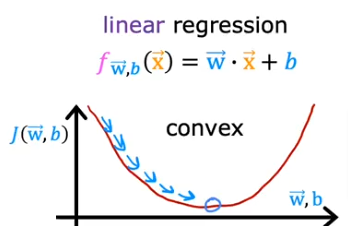
Linear Regression
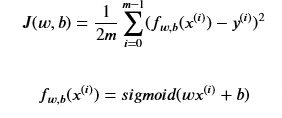
Recall the LR squared error cost function is a way to measure how well the parameters fit a model
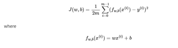
where m = number of training examples
n is the number of features
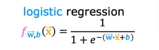
Logistic Regression
- If we use the same formula, it will plot to a non-convex curve which will not work to find the minimum loss value
- So we have to use something else which is called the Logistic Loss Function
Cost Logistic Function
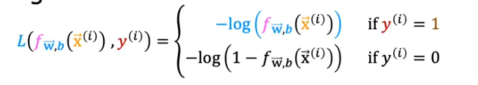
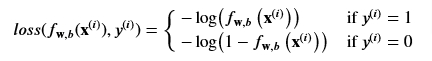
Loss Function
Loss is a measure of the difference of a single example to its target value
- If you remember that the cost is the summation of the losses for each predicted value
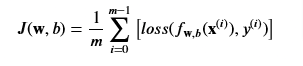
Cost Function
Cost is a measure of the losses over the training set
- So the Cost for the Logistic Regression will be the summation of all the losses
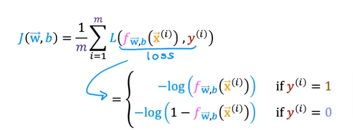
- If the label y(i) =1 it will be the first formula, and if y(i) =0 it will be the second
- Let’s focus on the first line above where y=1
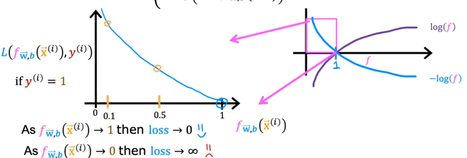
- Loss is lowest when f(x) predicts values close to y, so as the value is close to 1 the value if close to 0, and as f(x) approaches 0 the loss becomes close to infinity
- Let’s focus now on when the value is close to 0, the second part of the equation
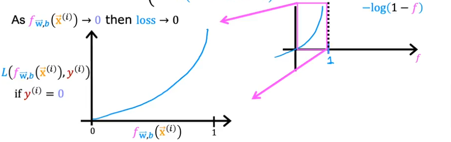
- When the loss is 0 or close to 0, the loss will be very small
- And as it turns out the curve will be convex once we sum it all up
Simplified Loss
Combine the two together to form one simple formula
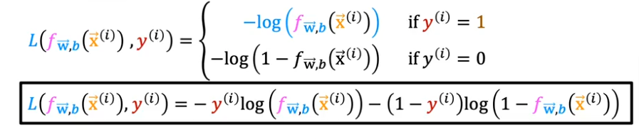
- Remember that it is just the above two combined into one
- consider y(i) can have only two values, 0 and 1
- once y(i)=0 the left hand is eliminated
- once y(i) =1 the right hand is eliminated
Simplified Cost
So from the loss function above we can sum up all the loss functions and it’ll add up to the cost function

Code
x_train = np.array([0., 1, 2, 3, 4, 5],dtype=np.longdouble)
y_train = np.array([0,  0, 0, 1, 1, 1],dtype=np.longdouble)
plt_simple_example(x_train, y_train)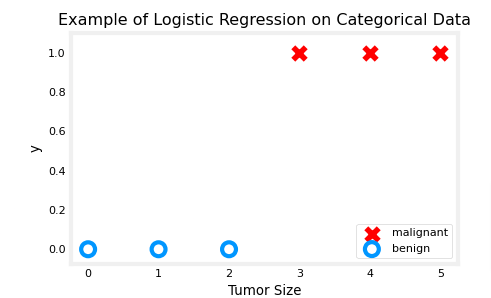
Plot squared error
plt.close('all')
plt_logistic_squared_error(x_train,y_train)
plt.show()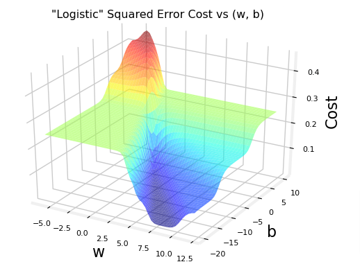
As you can see it is not convex nor is it smooth so it will be hard to find the minimal loss value. Now let’s look at the
Logistic Loss Function
plt_two_logistic_loss_curves()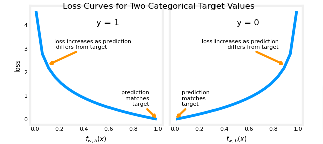
- The sigmoid output is between 0 and 1
Simple Loss Function
We can combine the two into one formula so we can apply to the entire dataset and it would be easier to fit the gradient descent function

- Remember that it is just the above two combined into one
- consider y(i) can have only two values, 0 and 1
- once y(i)=0 the left hand is eliminated
- once y(i) =1 the right hand is eliminated
plt.close('all')
cst = plt_logistic_cost(x_train,y_train)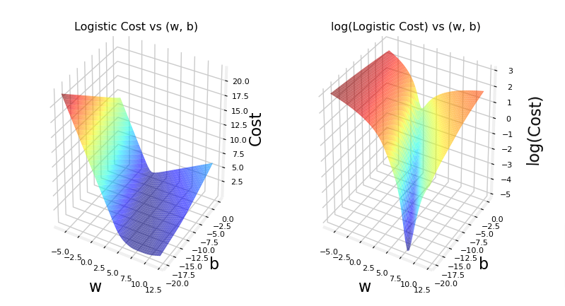
Cost Function
The cost function as you recall is the summation of the loss values
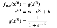
and the simplified loss function can be substituted

and since we are working with Logistic Regression our sigmoid function is g(z)
import numpy as np
%matplotlib widget
import matplotlib.pyplot as plt
from lab_utils_common import  plot_data, sigmoid, dlc
plt.style.use('./deeplearning.mplstyle')
X_train = np.array([[0.5, 1.5], [1,1], [1.5, 0.5], [3, 0.5], [2, 2], [1, 2.5]]) #(m,n)
y_train = np.array([0, 0, 0, 1, 1, 1]) #(m,)# we'll use a helper function to plot
fig,ax = plt.subplots(1,1,figsize=(4,4))
plot_data(X_train, y_train, ax)
# Set both axes to be from 0-4
ax.axis([0, 4, 0, 3.5])
ax.set_ylabel('$x_1$', fontsize=12)
ax.set_xlabel('$x_0$', fontsize=12)
plt.show()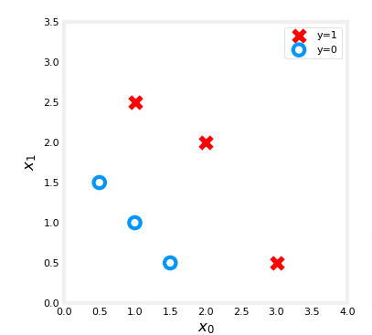
Cost Function
Formula is above
The algorithm for compute_cost_logistic loops over all the examples calculating the loss for each example and accumulating the total.
Note that the variables X and y are not scalar values but matrices of shape (𝑚,𝑛m,n) and (𝑚𝑚,) respectively, where 𝑛𝑛 is the number of features and 𝑚𝑚 is the number of training examples.
def compute_cost_logistic(X, y, w, b):
    """
    Computes cost

    Args:
      X (ndarray (m,n)): Data, m examples with n features
      y (ndarray (m,)) : target values
      w (ndarray (n,)) : model parameters
      b (scalar)       : model parameter

    Returns:
      cost (scalar): cost
    """

    m = X.shape[0]
    cost = 0.0
    for i in range(m):
        z_i = np.dot(X[i],w) + b
        f_wb_i = sigmoid(z_i)
        cost +=  -y[i]*np.log(f_wb_i) - (1-y[i])*np.log(1-f_wb_i)

    cost = cost / m
    return cost
Check the value
w_tmp = np.array([1,1])
b_tmp = -3
print(compute_cost_logistic(X_train, y_train, w_tmp, b_tmp))
Vary w
Now, let’s see what the cost function output is for a different value of 𝑤w.
- In a previous lab, you plotted the decision boundary for 𝑏=−3,𝑤0=1,𝑤1=1b=−3,w0=1,w1=1. That is, you had
b = -3, w = np.array([1,1]). - Let’s say you want to see if 𝑏=−4,𝑤0=1,𝑤1=1b=−4,w0=1,w1=1, or
b = -4, w = np.array([1,1])provides a better model.
Let’s first plot the decision boundary for these two different 𝑏b values to see which one fits the data better.
- For 𝑏=−3,𝑤0=1,𝑤1=1b=−3,w0=1,w1=1, we’ll plot −3+𝑥0+𝑥1=0−3+x0+x1=0 (shown in blue)
- For 𝑏=−4,𝑤0=1,𝑤1=1b=−4,w0=1,w1=1, we’ll plot −4+𝑥0+𝑥1=0−4+x0+x1=0 (shown in magenta)
import matplotlib.pyplot as plt

# Choose values between 0 and 6
x0 = np.arange(0,6)

# Plot the two decision boundaries
x1 = 3 - x0
x1_other = 4 - x0

fig,ax = plt.subplots(1, 1, figsize=(4,4))
# Plot the decision boundary
ax.plot(x0,x1, c=dlc["dlblue"], label="$b$=-3")
ax.plot(x0,x1_other, c=dlc["dlmagenta"], label="$b$=-4")
ax.axis([0, 4, 0, 4])

# Plot the original data
plot_data(X_train,y_train,ax)
ax.axis([0, 4, 0, 4])
ax.set_ylabel('$x_1$', fontsize=12)
ax.set_xlabel('$x_0$', fontsize=12)
plt.legend(loc="upper right")
plt.title("Decision Boundary")
plt.show()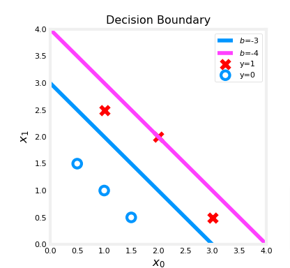
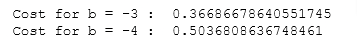
You can see from this plot that b = -4, w = np.array([1,1]) is a worse model for the training data. Let’s see if the cost function implementation reflects this.
w_array1 = np.array([1,1])
b_1 = -3
w_array2 = np.array([1,1])
b_2 = -4

print("Cost for b = -3 : ", compute_cost_logistic(X_train, y_train, w_array1, b_1))
print("Cost for b = -4 : ", compute_cost_logistic(X_train, y_train, w_array2, b_2))