~\AI\ML\Stanford_Ng>py -m venv mlvenv
~\AI\ML\Stanford_Ng>mlvenv\Scripts\activate

(mlvenv) ~\AI\ML\Stanford_Ng>pip install ipykernel
(mlvenv) ~\AI\ML\Stanford_Ng>python -m ipykernel install --user --name=mlvenv --display-name "ML venv"Linear Regression
My thanks and credit to Stanford University & Andrew Ng for their contributions.
Recap
Most of what follows is basic math most of us learned long ago, so here is a refresher: Remember regression analysis is part of Supervised Learning:
Regression is the relationship between a dependent and an independent variable. The dependent variable is a continuous variable that we want to predict, and the independent variables are the variables that, we believe, influence the value of the dependent variable. The inputs X are used to predict an infinite number/value for us. We only provide the input and expect the model to provide a prediction
Regression techniques are used for predicting a continuous value. For example, predicting the price of a house based on its characteristics or estimating the CO2 emission from a car’s engine.
To begin, consider the following scatter plot.
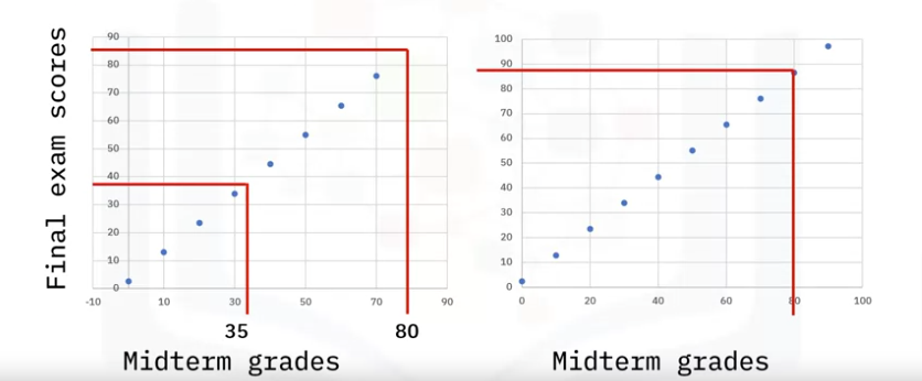
- Assume you have midterm grades on the x-axis,
- final grades on the y-axis, and
- you have plotted the points associated with each grade.
Now, you want to know the final exam scores of students who had a score of 35 on their midterm.
- You can guess that their final score will be very close to 40.
- What if you wanted to guess a final score for a student whose midterm grade falls outside the range of the plotted points? Say, a student who got 80?
- Basically, you can fit a line through the data and make an educated guess for values within or outside the range of the data set.
A linear regression model is designed to predict the Target Value/Column given the Data Input/Column
Terminology
The following explanations will be used throughout AI and pretty basic depending on your background, but let’s cover it anyways:
- Input : x - midterm grades below, are called input variable or feature are lower case x
- Output: y - final exam scores below, are called output variable or target variable and are lower case y
- So when the data is given in a table format, the first column would be Midterm grades and the second column would be Final exam scores
- Each row in the table represents an x and y value and is called a training example
- A single training example is represented as (x,y)
- The total number of rows in the dataset is named: m = number of trainig examples
- To target a specific training example we specify the row number with a superscript like this: ( x(i), y(i)quarto render) = ith training example with i = to any number in the length of the dataset m or the row number in the table. If i=2 it means we are addressing row 2
- So when we mention that we provide a training set to our model means we provide both the features and targets
Code
Setup
- Before we get started let’s setup a venv named: mlvenv
- Reason being is I want to isolate all the ml information from Stanford/Ng in one place
- Create the venv
- Activate it
- We install an ipykernel so we can access it from within jupyter notebook
- Register the mlvenv Kernel and assign a name inside jupyter notebook to use
- We’ll import what we need and assign the plot styles to a style sheet we’ve included in the same directory
import numpy as np
import matplotlib.pyplot as plt
plt.style.use('./deeplearning.mplstyle')
So let’s say we want to guess what the sales price of a house would be based on square feet, and we have the following data
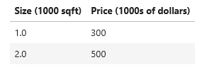
- Let’s store the data in one-dimensional NumPy arrays
- we’ll name the first column as x_train (as it stands for training data), we will train the algorithm on this data so it can predict the price given size later
- we’ll name the second column as y_train and save both in their arrays
# x_train is the input variable (size in 1000 square feet)
# y_train is the target (price in 1000s of dollars)
x_train = np.array([1.0, 2.0])
y_train = np.array([300.0, 500.0])
print(f"x_train = {x_train}")
print(f"y_train = {y_train}")
x_train = [1. 2.]
y_train = [300. 500.]Number of Training Examples
- As we mentioned above m is the total number of training sets
- we can use .shape() which is a tuple and extract the first object with .shape[0] to retrieve that
- or we can use the len() function
m = x_train.shape[0]
mm = len(x_train)
print(f"Number of training exampales is from shape[0] = {m} or from len() = {mm}")
Number of training exampales is from shape[0] = 2 or from len() = 2You will use (x(i), y(i)) to denote the ith training example. Since Python is zero indexed, (x(0), y(0)) is (1.0, 300.0) and (x(1), y(1)) is (2.0, 500.0).
To access a value in a Numpy array, one indexes the array with the desired offset. For example the syntax to access location zero of x_train is x_train[0]. Run the next code block below to get the ith training example.
i = 0 # Change this to 1 to see (x^1, y^1)

x_i = x_train[i]
y_i = y_train[i]
print(f"(x^({i}), y^({i})) = ({x_i}, {y_i})")
(x^(0), y^(0)) = (1.0, 300.0)Plot
# Plot the data points
plt.scatter(x_train, y_train, marker='x', c='r')
# Set the title
plt.title("Housing Prices")
# Set the y-axis label
plt.ylabel('Price (in 1000s of dollars)')
# Set the x-axis label
plt.xlabel('Size (1000 sqft)')
plt.show()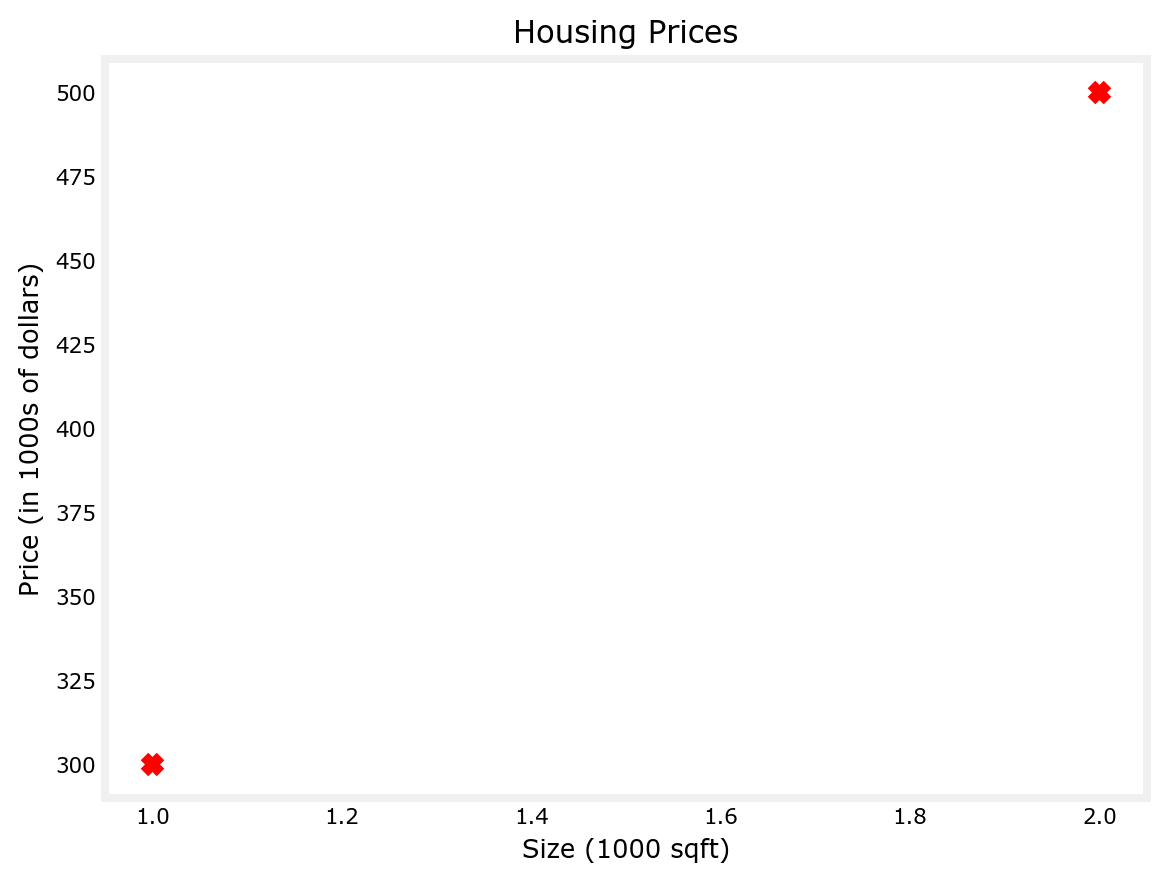
Linear Regression
A sdimple straight line is the most likely the most well known model in the world. Linear regression models the relationship between one or more independent variables, and one dependent variable, by finding the best-fit line for the data set. The ideal model would minimize the sum of squared errors.
Simple Example
Here is our simple, one feature, straight line, linear regression model
- In order to plot it we need to guess the values of w & b then use the training data to see how close to the actual data it is
- So let’s choose w=100 and b=100
- For loop: this is not the most efficient way to calculate the linear regression, but since we only have 2 training sets it will do the trick for now. I’ll cover the vector method later
- Define a function that will calculate the linear regression and name it: comput_model_output()
- Guess values for w & b and plot
- As you see below, the guess for w & b yield a bad fitting line
- Change w & b till you come up with w=200 and b=100 which will fit the two points perfectly
def compute_model_output(x, w, b):
    """
    Computes the prediction of a linear model
    Args:
      x (ndarray (m,)): Data, m examples
      w,b (scalar)    : model parameters
    Returns
      y (ndarray (m,)): target values
    """
    m = x.shape[0]
    f_wb = np.zeros(m)
    for i in range(m):
        f_wb[i] = w * x[i] + b

    return f_wb
# Set w and b and call the function to calculate it, then plot the results
w = 100
b = 100
tmp_f_wb = compute_model_output(x_train, w, b,)
# Plot our model prediction
plt.plot(x_train, tmp_f_wb, c='b',label='Our Prediction')
# Plot the data points
plt.scatter(x_train, y_train, marker='x', c='r',label='Actual Values')
# Set the title
plt.title("Housing Prices")
# Set the y-axis label
plt.ylabel('Price (in 1000s of dollars)')
# Set the x-axis label
plt.xlabel('Size (1000 sqft)')
plt.legend()
plt.show()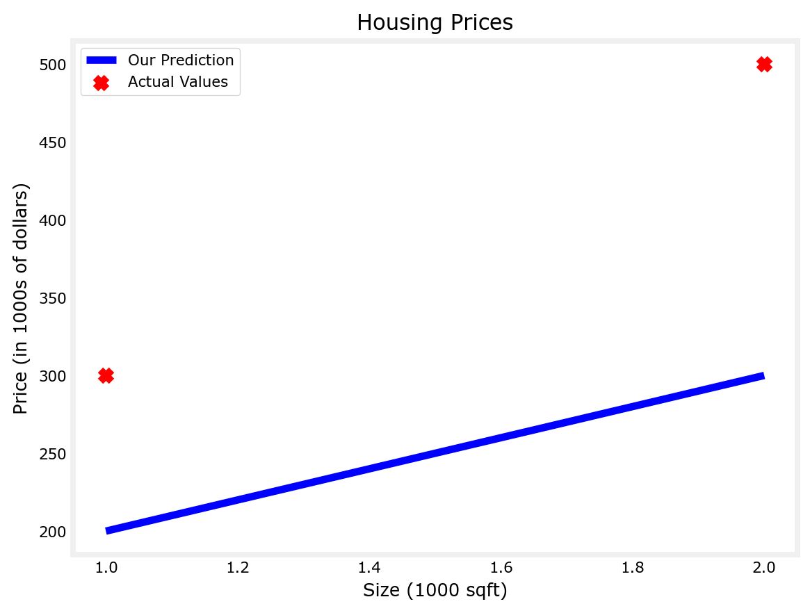
One Variable
Let’s say you want to predict the price of a house based on the ft2. Let’s plot the data from the table and we have
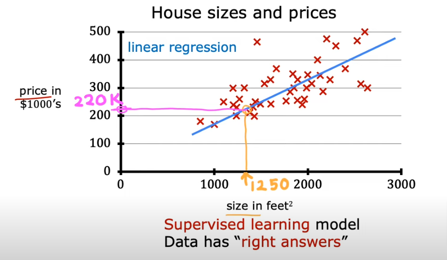
Here is a general overview of the lR model:
- You start with a training set with features and targets
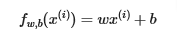
- You feed the training set to the learning algorithm, let’s call it model: f
- So we are inputing the feature into f and we want f to output the prediction of y, or the estimated \(\hat{y}\)
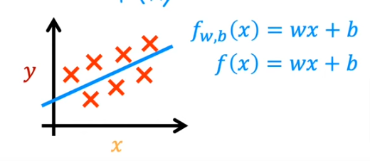
- So we represent the function f as: f(w,b)=wx + b or as a shortcut: f(x)
- So we are using a straight line to make prediction, the most simple models you can look at
- Therefore it is called Linear Regression with One Variable (Univariable)
Line of Best Fit
This line is called the line of best fit.
Simply put, regression is the relationship between a dependent and independent variable. In regression, the dependent variable is a continuous variable.
- Looking at our line again, you can use a formula to predict values that are not accounted for.
- The formula for this line is y equals m x plus b.
- “m” is the slope of the line calculated as rise over run.
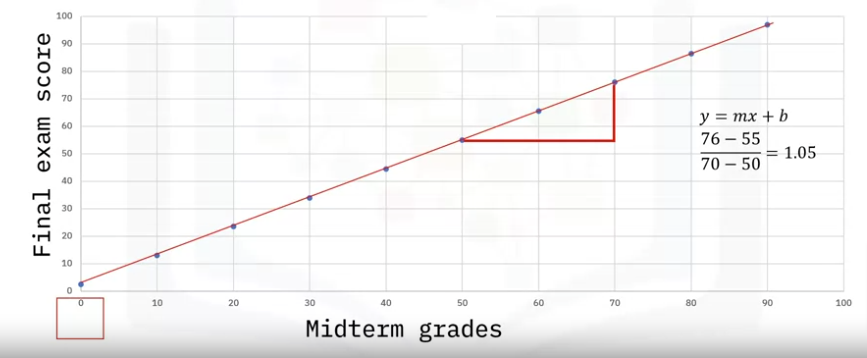
Let’s calculate m.
- Rise, in this case, will be 76 minus 55 divided by run, which is 70 minus 50. That will give us 1.05. This means that for every 1 mark increase in a midterm grade, the final exam score will increase by 1.05.
- B is the y-intercept, that is, where the line meets the y-axis. Mathematically speaking, it is the value of y when x is 0.
- If you substitute x as zero into the “y equals m x plus b” equation, you will see that the y-intercept is 2.5.
- This means that even if a student gets a 0 on the midterm, they will still get a 2.5 on the final exam.
The example above is a linear relationship between the dependent and independent variable, which is the simplest form of regression. Sometimes you may have multiple independent variables predicting your dependent variable.
So how do we know that we have a line of best fit? This is where the Cost Function comes in. I’ll cover that in the next page
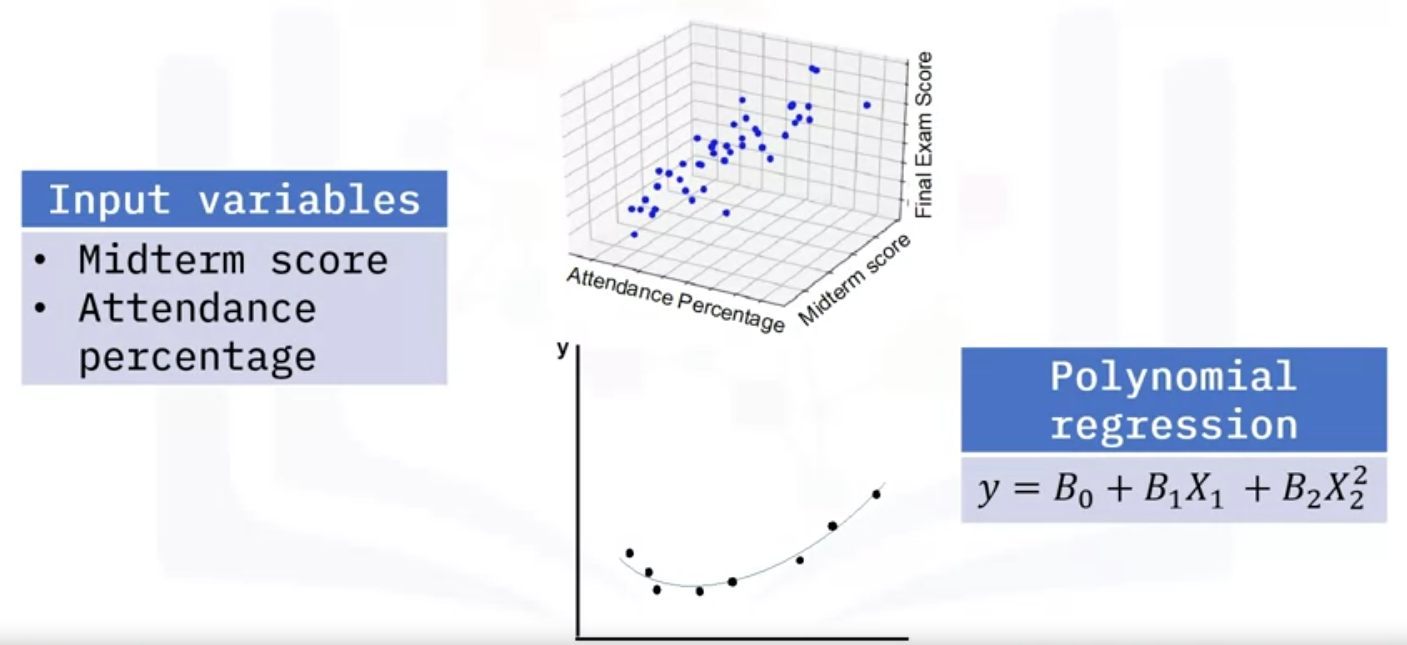
Polynomial Regression
In the final exam problem, you can have more variables that predict the outcome of the final exam score.
- You may have two variables instead, such as midterm score and attendance percentage.
- In this case, you would be dealing with a 3D graph with two slopes:
- one for the relationship between midterm score and final score,
- and one for attendance percentage and final score.
- imagine you have 10 variables.
- This model uses a polynomial of degree two to account for the nonlinear relationship.
Regularized Regression
When you want to avoid too much reliance on the training data, you can use regularized regression, such as Ridge, Lasso, and ElasticNet. The main idea here is to constrain the slope of the independent variables to zero by adding a penalty.
Ridge regression
Shrinks the coefficients by the same factor but doesn’t eliminate any of the coefficients.
Lasso regression
Shrinks the data values toward the mean, which normally leads to a sparser model and fewer coefficients.
ElasticNet regression
Is the optimal combination of Ridge and Lasso that adds a quadratic penalty.
The following are popular examples of advanced regression techniques.
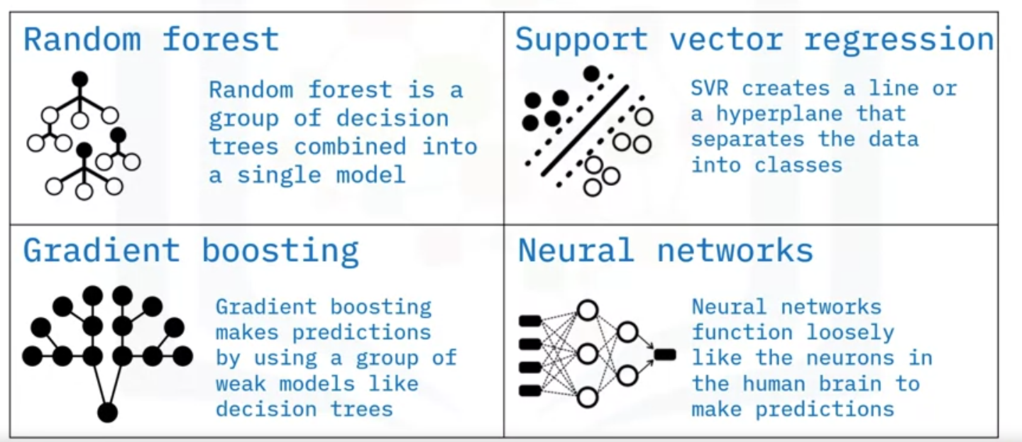
Random forest
Random Forest is a group of decision trees combined into a single model.
Support vector regression, or SVR
SVR creates a line or a hyperplane that separates the data into classes.
Gradient boosting
Gradient boosting makes predictions by using a group of weak models like decision trees.
Neural networks.
The idea behind neural networks is inspired by the neurons in the brain used to make predictions.
Summary
We covered Classification models in Supervised Learning in ML/Basics. Here is a reminder:
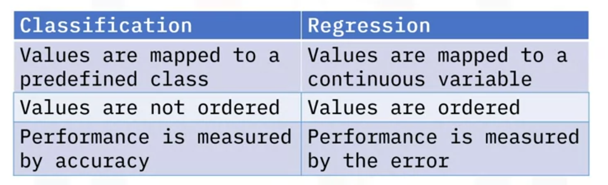
Here are some differences between classification and regression.
- Classification works with classes such as ”Will I pass or fail?” or “Is this email spam or not spam?”
- Regression is mapped to a continuous variable.
- In classification, values are not ordered, as belonging to one class doesn’t necessarily make a value more or less superior.
- In regression, values are ordered, and higher numbers have more value than lower numbers.
- You use accuracy to measure the performance of a classification algorithm, that is, how many you predicted correctly from the total population.
- In regression, you use the error term, that is, how far away you were from the actual predictions.